div class=”ChapterContextInformation”>
17. Computational Fluid Dynamics for Evaluating Hemodynamics
Keywords
HemodynamicsVelocity fieldPressure mapsWall shear stressStreamlinesOverview
Blood flow in vessels plays an important role in the physiological response of the vasculature in health and disease and in preserving the function of the end organs. While many of the descriptors that are important in evaluating the health of a vascular territory are well established, many others remain the domain of active investigation. The ability to establish the relationship between adverse hemodynamics and patient outcome has dramatically improved with the advent of robust high-resolution, noninvasive imaging measures of the local disease in the vessel wall, the prevailing flow conditions, and the status of the end organ. However, establishing causal connections between hemodynamic descriptors and physiological impact requires detailed knowledge of the spatial and temporal distribution of those descriptors. Computational Fluid Dynamics (CFD) methods are well suited to this task. The ever-increasing power of computational platform resources permits simulations of appropriately complex anatomic models in manageable compute times. In this chapter, the assumptions that underlie the CFD modeling approaches that are widely used in describing flow in the human vasculature are discussed. A description will be provided of the computational pipeline. Finally, examples of applications to patient-specific conditions will be presented.
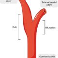
Assessing the Velocity Field

A color-coded CFD-computed velocity field with high velocities encoded in red for a schematic representation of the extracranial carotid bifurcation. Slow recirculating flow in the bulb can be observed (blue region). A plot of the derived wall shear stress along the lateral wall of the internal carotid artery shows an extended area of low wall shear stress in the bulb from the point of flow separation (S) to reattachment (R)
More recently, advances in computational methods have been included into commercial solvers with much of that development being spurred by applications to the aerospace, auto, and other industries where flow conditions are significantly more extreme than in the human vasculature. These solvers are now sufficiently sophisticated to readily incorporate realistic geometries and physiological flow conditions and can therefore be applied to patient-specific anatomy and flow.
Imaging Approaches
The interest in utilizing CFD methods in considerations of hemodynamics in vascular disease is manifold. While there are a variety of methods for assessing important features of hemodynamics in vivo, these have relatively coarse spatial and temporal resolution and suffer from technical and physiological challenges. Ultrasound is noninvasive and relatively inexpensive and has excellent temporal resolution for determining the full spectrum of velocities in a fixed insonation volume. It has strong abilities for quantifying peak velocities in flow jets which can be used to infer the degree of stenosis. It is unable to similarly map the velocity field through a three-dimensional volume and, in many cases, is obscured by bowel gas, calcifications, or overlying bone – as is the case for the brain. Furthermore, it is highly operator-dependent and is unsuited to measurement of volume flow. Catheter-injected angiography provides qualitative visualization of flow dynamics which is important for determining important physiological features such as vascular patency and the existence of collateral pathways. However, it is invasive and expensive and is not quantitative. MR imaging, particularly 4D Flow, has a number of desirable features: it is noninvasive and can depict the velocity field in space and time without limitations of overlying anatomy [7, 8]. This offers the possibility of determining derived descriptors such as volume flow and wall shear stress, the frictional force exerted by blood on the vessel wall. However, MR has moderate spatial and temporal resolution. Unlike ultrasound which determines the spectrum of velocities in the insonation volume, MR provides a voxel-averaged velocity measurement. Because of practical imaging constraints such as signal to noise ratios and acquisition times (which are often longer than 10 minutes), studies in a number of vascular territories are acquired with less than three or four voxels across the vascular lumen. The derivation of critical parameters such as the wall shear stress rely on an accurate measurement of the spatial gradient of velocities at the vessel wall, and MR-derived estimates of these measures must therefore be viewed with appropriate caution. A major attraction of CFD methods is the ability to specify very high resolution in space and time and calculate velocity fields with resolution far beyond anything that is currently achievable with in vivo imaging methods.
Computational Fluid Dynamics (CFD)
In most vascular territories and under a broad range of healthy and pathologic states, a numerical solution of the Navier-Stokes equations can be attained with limited and reasonable assumptions. While methods exist to accommodate each of the following, they are often neglected in conventional CFD calculations of hemodynamics: the vessel wall is assumed to be rigid; blood is assumed to be a Newtonian fluid; and blood flow is considered to be laminar without the presentation of turbulence. With those assumptions, CFD calculations can be conducted if the surface boundary of the vascular structure of interest is specified, if the inlet flow waveform is defined, and if the outlet flow conditions are appropriately conditioned.
Vascular Compliance
Returning to the major assumptions, the importance of neglecting vascular compliance is not fully understood given the difficulty in conducting a simulation that includes wall motion – a so-called fluid-structure interaction (FSI) problem [9]. Results of FSI compared to CFD with rigid walls indicate that neglecting compliance in a number of vascular territories (such as the intracranial vessels) has little effect [10]. In other territories such as the aorta, larger differences are reported [11]. It is, however, difficult to assess the extent to which the wall motion is correctly incorporated into the FSI models given their reliance on unreliable in vivo imaging to condition their boundary values. Furthermore, in conditions such as atherosclerosis, aneurysmal disease, or in the elderly population in general, resorting to an FSI simulation is likely unwarranted since vessels lose their compliance under those conditions, and conventional CFD methods are likely to suffice.
Newtonian Viscosity
Fluid viscosity describes how the shear stress varies with changes in the shear rate, and if shear stress changes linearly with shear rate, the viscosity is constant. It is then referred to as a Newtonian fluid. Most CFD models assume that blood is a Newtonian fluid. There are in vivo situations where this condition is violated. On one limit, when blood recirculates slowly, red blood cells can aggregate, resulting in an increase in viscosity. Regions of slowly recirculating flow can occur in regions of aneurysmal dilatation. There are a number of analytical formulas that can be incorporated into CFD solvers that attempt to provide more physical models of blood viscosity at low shear rates [12]. There are reports that these effects are relatively small. On the other limit, the viscosity of blood decreases substantially when passing through narrow (<300 micron) vessels when red blood cells move to the center of the vessel leaving only plasma near the wall of the vessel (the Fåhraeus–Lindqvist effect). These vessels are of the scale of arterioles and capillaries and are generally not of current interest for the determination of detailed features in their velocity fields.
Turbulence
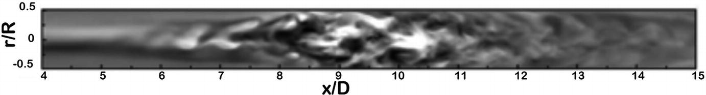
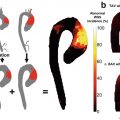
A DNS simulation of flow in the longitudinal plane of a tube with a non-stenosed diameter D, and a 75% eccentric stenosis by area. Streamwise velocity fluctuations are shown (x) along the length of the vessel (x) between 4 and 15 diameters distal to the stenosis. This map shows the transition from regular to complex flow as the flow jet breaks into vortical eddies. (Varghese et al. [14], reproduced with permission)
In general, many physiological conditions of interest can be closely approximated by laminar flow through rigid-walled vessels with Newtonian viscosity. For those cases, conventional CFD simulations can then be applied to generate highly accurate estimates of the velocity field. However, in cases where those conditions are not met, in vivo imaging modalities, in particular 4D Flow MRI methods, provide the intriguing prospect of more accurately determining the velocity field than is possible with CFD as the true physiological behavior is inherently present on a patient-specific basis, and does not require modeling. In the remainder of this chapter, we will restrict ourselves to a discussion of the application of conventional CFD to the analysis of hemodynamics in vivo.
CFD in the Laminar Flow Regime
A CFD analysis provides a numerical solution of the Navier-Stokes equations, the governing equations of fluid motion. The key components required as input to the numerical model are a description of the lumenal surface of the vessels of interest and specification of the inlet and outlet flow boundary conditions.
Lumen Surface
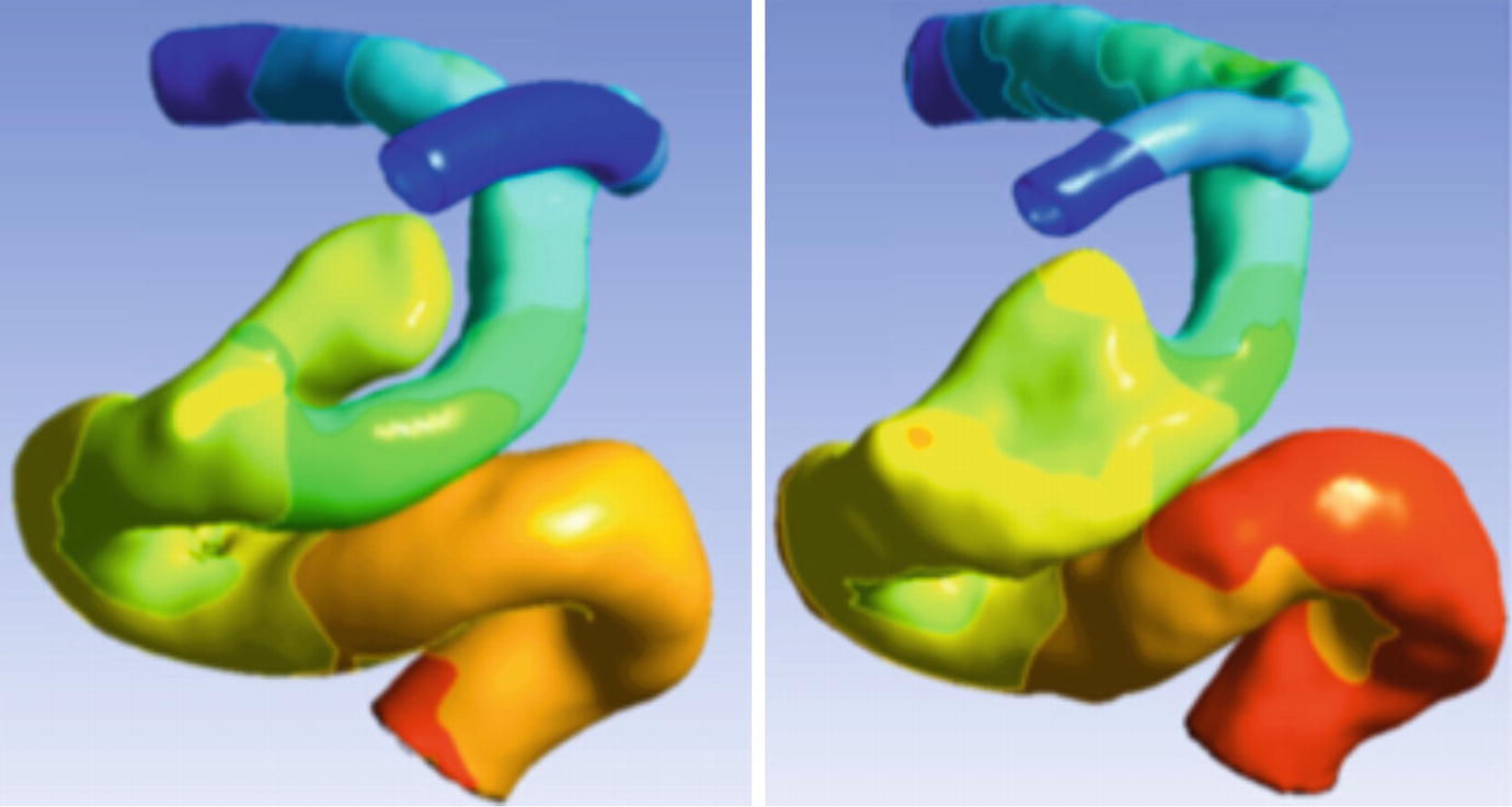
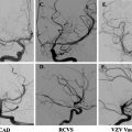
Impact of acquisition resolution. CFD -calculated pressure distribution in a distal internal carotid artery with a cavernous segment aneurysm. Left: pressure map using surface segmentation from a rotational DSA study with 0.2 mm isotropic resolution clearly shows the separation between distal ICA and the aneurysm. Right: pressure map using surface segmentation from a CE-MRA study with 0.7 mm isotropic resolution fails to correctly resolve the inferior aspect of the aneurysm
Related posts:

Stay updated, free articles. Join our Telegram channel

Full access? Get Clinical Tree


