Fig. 1.
Three components for an in-vivo assessment tool are pre-strain measurement, inverse model and population average fiber architecture of valve leaflets
2 Methods
To demonstrate the ideal capabilities of our approach, we utilized archival quality in-vitro experimental data from pericardial bioprosthetic heart valve to develop the parameter estimation tool based upon inverse modeling. The leaflets were imaged at three different static transvalvular pressures using surface markers and dual-camera setup [1] (Fig. 2). Leaflets were then removed and their fiber architecture was determined using light scattering technique [2]. Then the leaflets were dissected and put under biaxial test to determine their stress-strain relationship. This highly comprehensive data set with high resolution, marker positions at multiple pressures, valve specific fiber architecture and biaxial data was ideal for this study – to design the inverse model, validate it and calculate its sensitivity to various input parameters and optimization constraints. There is no existing method for inverse modeling of heart valves as per authors’ knowledge. This is due to the difficulty in modeling them as well as their small size and thickness and fast movement in-vivo, leading to poor quality of imaging.


Fig. 2.
The experimental setup to obtain valve shape in-vitro at different transvalvular pressure levels
2.1 The Forward Model
Each of the valve leaflet was modeled as a thin shell and the contact between leaflets was treated using the augmented Lagrange multiplier method. The basal attachment was fixed as in the experiments and a normal pressure on the leaflets was applied linearly increasing upto 120 mm of Hg. The forward model was implemented in FEBio [3] using quadrilateral shell elements using quasi-static solver. The shape of the valve was provided by Edwards in the form of a quadrilateral meshed geometry file, where each leaflet was made up of 1025 cells and 1082 nodes. To improve the refinement as well as quality of elements, the geometry was imported into Hypermesh and remeshed with each leaflet made up of 2789 cells and 2880 nodes. Leaflets were discretized using four node quadrilateral elements, with each node assigned six degrees of freedom (three for translation and three for rotation). Therefore, the complete discrete version of the model had 51,840 degrees of freedom. A constant thickness was assigned to each leaflet as measured during the experiment. The stresses were integrated through the shell thickness using 3 point Gauss quadrature rule to obtain bending moments. To map the fiber architecture from two-dimensional output of the above-mentioned experimental method onto the three-dimensional valve structure, a spline-based technique previously developed was used [4].
2.2 The Material Model
The valve tissues are made up of multiple layers (fibrosa, ventricularis etc.) with different types of fibers embedded in a matrix for each of them [5, 6]. However it is very hard to take into account the contribution of each layer separately. Therefore, here we take one of the most realistic material models developed – where tissue is idealized as a planar network of collagen fibers (main load bearing component) embedded in a ground substance (glycosaminoglycans, elastin, water) [7]. Thus, the strain energy is assumed to be a sum of the contributions from fibrillar (anisotropic) and non-fibrillar (isotropic) components expressed in terms of the tissue level Green-Lagrange strain  :
:

Here  and
and  are strain energy functions representing ground-matrix and fiber contributions respectively. The ground-matrix function describes low-strain behavior and provides stiffness in the unloaded state. Tissue response to large strains is accommodated by the anisotropic term characterizing the fibrillar microstructure averaged through the thickness. The isotropic contribution is assumed to be neo-Hookean. Following the formulation in [7], the ensemble
  Piola-Kirchhoff stress in a single fiber is

where,  is the fiber stiffness, D is the fiber recruitment function and
  is the uniaxial Lagrangian strain in single fiber aligned in direction
  so that
  . However, in present formulation, to avoid extremely high computational times, a simplified model was used [8], where the integral is approximated as an exponential function:

The important aspect of this approach is that it allows us to reduce the number of unknown material parameters in fiber component to only two, thus, reducing the computational time in determining them. The matrix component was modeled as a compressible neo-Hookean material and the properties were borrowed from flexural testing results previously published. For a distribution of fibers in a planar biaxial state, we get the planar stress by integrating over the distribution

The fiber distribution  was determined at every point of the tissue using SALS setup [2] and approximated as a normalized Gaussian distribution. For the matrix part
  , a neo-Hookean model was used for which there parameters were estimated from flexural studies previously conducted.
 :
:
(1)
 and
and  are strain energy functions representing ground-matrix and fiber contributions respectively. The ground-matrix function describes low-strain behavior and provides stiffness in the unloaded state. Tissue response to large strains is accommodated by the anisotropic term characterizing the fibrillar microstructure averaged through the thickness. The isotropic contribution is assumed to be neo-Hookean. Following the formulation in [7], the ensemble
  Piola-Kirchhoff stress in a single fiber is
(2)
 is the fiber stiffness, D is the fiber recruitment function and
  is the uniaxial Lagrangian strain in single fiber aligned in direction
  so that
  . However, in present formulation, to avoid extremely high computational times, a simplified model was used [8], where the integral is approximated as an exponential function:
(3)

(4)
 was determined at every point of the tissue using SALS setup [2] and approximated as a normalized Gaussian distribution. For the matrix part
  , a neo-Hookean model was used for which there parameters were estimated from flexural studies previously conducted.
2.3 The Algorithm
The above forward model was put in an optimization loop where the parameters were initialized with a guess and solution was iterated until convergence was achieved. The objective cost function was defined as the difference in shape of the deformed mesh and that of the experimental data points. The difference was calculated along the normal direction of deformed mesh. Thus, it can be defined mathematically as

where,  are the input points from experiment and
  are their projection on deformed valve surface obtained from the forward model with material parameters
  . It should be noted that the above cost function does not use the information about experimental data points being the material points. Instead, the points were used only to describe valve shape. This was done to be consistent with the clinical imaging modalities (e.g. ultrasound) which provides only the shape without any information about material points. The minimization of above defined cost function is a highly non-linear function because of the contact constrained between leaflets. The non-linear least squares problem of minimizing the cost function was solved using Levenberg-Marquardt algorithm:

(5)
 are the input points from experiment and
  are their projection on deformed valve surface obtained from the forward model with material parameters
  . It should be noted that the above cost function does not use the information about experimental data points being the material points. Instead, the points were used only to describe valve shape. This was done to be consistent with the clinical imaging modalities (e.g. ultrasound) which provides only the shape without any information about material points. The minimization of above defined cost function is a highly non-linear function because of the contact constrained between leaflets. The non-linear least squares problem of minimizing the cost function was solved using Levenberg-Marquardt algorithm:


