Functional MRI
Susie Y. Huang
Behroze Vachha
Steven M. Stufflebeam
Bruce R. Rosen
Bradley R. Buchbinder
Introduction
Since its inception, functional magnetic resonance imaging (fMRI) has attracted interest for its potential role in assisting the clinical diagnosis and management of patients who may have disruption of brain function due to pathologic conditions. Significant advancements have been made in applying fMRI to presurgical functional mapping in patients with structural brain lesions, including tumors, vascular malformations, epilepsy, and other lesions (1). The primary goal of presurgical planning using fMRI is to localize areas of eloquent cortex and associated white matter tracts in relation to lesions in order to avoid injury to critical functional areas during surgical resection.
This chapter provides a summary of the physiologic basis and biophysical principles of fMRI using the blood oxygen level-dependent (BOLD) effect, the main contrast mechanism used in nearly all clinical fMRI studies. We also discuss the practical concerns in clinical fMRI, including patient preparation, study design, image acquisition and processing, and data analysis and interpretation. We illustrate the utility of fMRI in presurgical planning through clinical cases. Finally, we address the potential challenges of clinical fMRI under pathologic conditions and anticipate future developments, including the most recent advancements in resting state fMRI.
Principles of BOLD fMRI
Physiologic Basis of BOLD fMRI
The interplay between neuronal activity, energy metabolism, and blood flow is central to understanding and interpreting fMRI. Although it was suggested more than a century ago that increased neural activity leads to increased regional cerebral blood flow (CBF) and cerebral blood volume (CBV) to meet metabolic demands, the complex biochemical and physiologic mechanisms underlying this process are still incompletely understood. For detailed discussion of the mechanisms involved, the reader is referred to the starred section “A basic model for the BOLD fMRI signal” (see later) as well as more complete texts on fMRI (2,3,4).
The general premise of the underlying physiology is as follows: the brain requires a continuous supply of glucose and oxygen to function, which is provided by CBF. Activated areas of the brain show increased glucose and oxygen metabolism and in turn increased CBF and CBV, which deliver the glucose and oxygen needed to meet metabolic demands. The oxygenation state of blood depends on the flow of blood into and out of a given volume of brain tissue as well as the rate of oxygen metabolism. At rest, the rate of oxygen consumption is matched to CBF, such that the fraction of oxygen extracted from blood remains relatively constant at approximately 40% throughout the brain (5). With neuronal activation, local increases in CBF and CBV increase the oxygenation state of blood and facilitate increased diffusion of oxygen from vessels to mitochondria within metabolically active cells. The CBF response overwhelms the demand for oxygen in the activated state (6,7), such that as blood flow increases, the fraction of oxygen that leaves the blood and is consumed by cells paradoxically decreases. As the delivery of oxygen by blood flow markedly increases while less oxygen is removed from the blood, the net effect is increased blood oxygenation in areas of brain activation. The increase in blood oxygenation with activation is the key physiologic underpinning of fMRI, as changes in the oxygen saturation of hemoglobin are responsible for the small changes in MR signal that are measured in BOLD fMRI.
Biophysical Principles of BOLD fMRI
The first demonstrations of functional MRI used dynamic susceptibility contrast from injected gadolinium-based contrast agents to track changes in CBF as a function of neuronal activation (8). Soon after these initial experiments, subsequent fMRI experiments (9) replaced the use of exogenous contrast agents with two endogenous contrast mechanisms: arterial spin-labeled flow contrast (10) and the intrinsic contrast arising from the local magnetic susceptibility changes induced by changes in the deoxyhemoglobin content of blood, that is, blood oxygen level–dependent (BOLD) contrast (11,12). Arterial spin labeling (ASL) alters the longitudinal magnetization of inflowing blood and creates contrast between the tagged longitudinal magnetization of inflowing arterial blood and stationary protons within the imaged volume. Because the functional sensitivity of ASL is lower than that of the BOLD method, ASL has found more limited application for fMRI than BOLD contrast, which is now by far the most commonly used contrast mechanism for fMRI and will be the focus of the remainder of this chapter.
The BOLD effect takes advantage of the intrinsic susceptibility contrast provided by blood in varying states of oxygenation. It was first observed in vitro by Thulborn et al. (12) and later demonstrated in vivo by Ogawa et al. (11,13), who applied BOLD contrast to the study of brain activation. BOLD imaging is based on the fact that deoxyhemoglobin, which is paramagnetic, changes the local magnetic field or susceptibility of capillaries and veins containing deoxygenated blood. Magnetic susceptibility represents the degree to which a material develops magnetization of its own when placed in an external magnetic
field. Paramagnetic substances such as deoxyhemoglobin strengthen the local magnetic field while diamagnetic substances such as oxyhemoglobin weaken the local magnetic field. The difference in magnetic susceptibility between deoxyhemoglobin within red blood cells and surrounding oxygenated tissue results in local magnetic field nonuniformity and a net reduction in the local MR signal, which is described as a T2* effect or reduction in the apparent transverse relaxation time. Conversely, as blood oxygenation increases, the local MR signal also increases.
field. Paramagnetic substances such as deoxyhemoglobin strengthen the local magnetic field while diamagnetic substances such as oxyhemoglobin weaken the local magnetic field. The difference in magnetic susceptibility between deoxyhemoglobin within red blood cells and surrounding oxygenated tissue results in local magnetic field nonuniformity and a net reduction in the local MR signal, which is described as a T2* effect or reduction in the apparent transverse relaxation time. Conversely, as blood oxygenation increases, the local MR signal also increases.
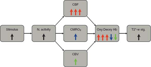 FIGURE 31.1 Schematic summary of key physiologic contributions to the T2*-weighted BOLD signal. Neural activity increases cerebral blood flow (CBF, red), cerebral metabolic rate of oxygen consumption (CMRO2, blue), and cerebral blood volume (CBV, green). Increased CBF delivers oxygen to the vessels, increasing the oxyhemoglobin to deoxyhemoglobin ratio (Oxy:Deoxy Hb). Increased CMRO2 extracts O2 from the vessels, decreasing the Oxy:Deoxy Hb ratio. Increased CBV augments the volume fraction of capillaries and venules more than arterioles, also decreasing the Oxy:Deoxy Hb ratio. On balance, the CBF increase is disproportionate to the CMRO2 and CBV increases, resulting in a net increased Oxy:Deoxy Hb ratio, decreased susceptibility-induced perivascular magnetic field perturbations, and increased T2*-weighted BOLD signal. |
Deoxyhemoglobin acts as an endogenous paramagnetic contrast agent in blood, which is modulated by variations in oxygen supply delivered by blood flow and oxygen consumption by tissue metabolism. In this simplified picture, neuronal activity leads to increased tissue metabolism, which in turn causes an increase in CBF to increase the delivery of oxygen (Fig. 31.1). As CBF increases to a greater extent than oxygen consumption, the fraction of oxygen that is extracted from blood decreases, and the blood becomes more oxygenated. The decrease in deoxyhemoglobin concentration leads to a small, but measurable, MR signal increase, which is in essence the BOLD effect.
It is generally accepted that brain activation, metabolic processes, and the hemodynamic response are coupled closely in both space and time. The BOLD signal is spatially mapped to functional areas of the brain through spatial encoding by magnetic field gradients following the principles of MR image formation. The temporal evolution of the BOLD signal in relation to neuronal activation also needs to be considered (Fig. 31.2). The BOLD hemodynamic response is relatively slow, evolving on the order of seconds, compared to the timescale of electrical activity in the brain, which is in the order of milliseconds.
Following the initial stimulus, some studies have shown a rapid initial decrease in signal intensity lasting 1 to 2 seconds called the “initial dip” (14,15,16,17), which is thought to reflect the initial increase in metabolic demand and increase in concentration of deoxyhemoglobin before the CBF response sets in. The early response is followed by a rise in the BOLD signal, peaking at about 5 to 6 seconds, due to the disproportionate rise in CBF and resulting decrease in concentration of deoxyhemoglobin. The BOLD signal gradually decreases and returns to baseline at about 10 seconds. A delayed undershoot of the signal below the baseline has been observed (17), reaching a minimum value at approximately 15 seconds. This “poststimulus undershoot” is hypothesized to result from hemodynamic and metabolic effects, including a slowly resolving CBV response (18,19), although the exact etiology remains unclear (17). The entire BOLD response can last longer than 20 seconds. The hemodynamic response is modeled as a mathematical function that can then be incorporated into the analysis of functional activation maps.
Following the initial stimulus, some studies have shown a rapid initial decrease in signal intensity lasting 1 to 2 seconds called the “initial dip” (14,15,16,17), which is thought to reflect the initial increase in metabolic demand and increase in concentration of deoxyhemoglobin before the CBF response sets in. The early response is followed by a rise in the BOLD signal, peaking at about 5 to 6 seconds, due to the disproportionate rise in CBF and resulting decrease in concentration of deoxyhemoglobin. The BOLD signal gradually decreases and returns to baseline at about 10 seconds. A delayed undershoot of the signal below the baseline has been observed (17), reaching a minimum value at approximately 15 seconds. This “poststimulus undershoot” is hypothesized to result from hemodynamic and metabolic effects, including a slowly resolving CBV response (18,19), although the exact etiology remains unclear (17). The entire BOLD response can last longer than 20 seconds. The hemodynamic response is modeled as a mathematical function that can then be incorporated into the analysis of functional activation maps.
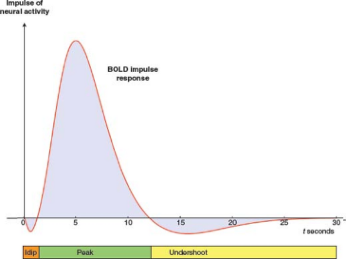 FIGURE 31.2 Schematic time course of the BOLD hemodynamic/metabolic impulse response. Vertical arrow represents a brief impulse of neural activity at time 0. Red curve represents a model for the time course of the BOLD impulse response. The time course is divided into three phases. (1) Some studies have observed an initial decrease in BOLD signal lasting 1 to 2 seconds, called the “initial dip.” It is likely due to a burst of oxidative metabolism that precedes the rise in CBF and associated influx of oxygen (15,16,17). (2) CBF subsequently increases disproportionately to CMRO2 and CBV, [dHb] declines, and the BOLD signal rises to a peak at about 5 to 6 seconds. As CBF and CMRO2 responses dissipate, the BOLD signal declines toward baseline. Later, the signal typically falls below baseline, forming a poststimulus undershoot which peaks at about 15 seconds, the origin of which remains controversial (17). The entire BOLD impulse response may last longer than 20 seconds. |
*A Basic Model for the BOLD fMRI Signal
A basic quantitative model helps to elucidate the physiologic and biophysical origins of the BOLD fMRI signal (2,17,20,21). Here, we outline a chain of reasoning that links activation-induced changes in blood flow, blood volume, and oxygen consumption to the magnitude of the T2*-weighted BOLD fMRI signal. While both gradient echo (GRE) and spin echo (SE) sequences can measure the BOLD effect, here we focus on the GRE sequence, which is preferred for most fMRI studies. Figures 31.3–31.9 illustrate the component principles. Numbered equations in the text link to the figures, and Figure 31.10 synthesizes the entire model.
The Balance between Oxygen Supply and Demand Modulates Capillary Venous Deoxyhemoglobin Concentration
The balance between oxygen supply and demand determines the degree of capillary venous oxygenation. The rate of oxygen supply increases in proportion to the rate of blood flow and the arterial oxygen concentration: CBF [O2]art. The rate of oxygen demand is the cerebral metabolic rate of oxygen consumption, CMRO2. The balance between oxygen supply and demand can be expressed by the oxygen extraction fraction (OEF), given by the ratio of the rate of consumption to the rate of delivery: OEF = CMRO2/(CBF [O2]art). Assuming that the arterial oxygen concentration is constant, and denoting OEF, CMRO2, and
CBF by E, M, and F, respectively, for brevity, we can summarize the balance between oxygen supply and demand by
CBF by E, M, and F, respectively, for brevity, we can summarize the balance between oxygen supply and demand by
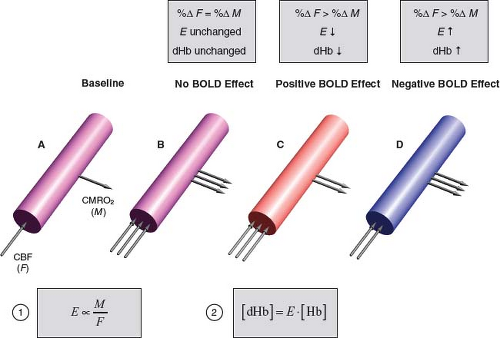 FIGURE 31.3 The balance between oxygen supply and demand modulates capillary–venous deoxyhemoglobin concentration (dHb). Oxygen supply is proportional to CBF (F). Oxygen demand is CMRO2 (M). The balance between oxygen supply and demand is reflected by the OEF (E) as the ratio M/F (Equation (1)). Assuming arterial blood is fully oxygenated, capillary-venous [dHb] is the total hemoglobin concentration ([Hb]) times the fractional deoxygenation (E) (Equation (2)). Cylinders represent a capillary or venule. Arrows schematically indicate different relative changes in CBF and CMRO2. Cylinder colors schematically indicate changes in [dHb] (inversely, O2 saturation). A: Baseline condition. Single arrows schematically indicate baseline CBF and CMRO2. Purple color indicates intermediate oxygen saturation. B: Outcome if neural activation were to cause equivalent relative increases in CBF and CMRO2 (%ΔF = %ΔM): OEF and [dHb] would be unchanged and there would be no BOLD effect. (Purple color indicates unchanged oxygen saturation.) C: Outcome when neural activation causes disproportionately greater increase in CBF than CMRO2 (%ΔF > %ΔM): OEF and [dHb] decrease, giving rise to the typical positive BOLD effect. Red color indicates increased oxygen saturation. D: Outcome if neural activation were to cause disproportionately greater increase in CMRO2 than CBF (%ΔF < %ΔM): OEF and [dHb] would increase, resulting in a negative BOLD effect. (Blue color indicates decreased oxygen saturation.) A negative BOLD effect can occur under some pathologic conditions, such as distal to a severe arterial stenosis (22,23,24) or in the presence of hemodynamic steal phenomenon associated with an arteriovenous malformation (25). The surprising fact that neural activation increases CBF disproportionately to CMRO2 undergirds the existence of BOLD fMRI. |
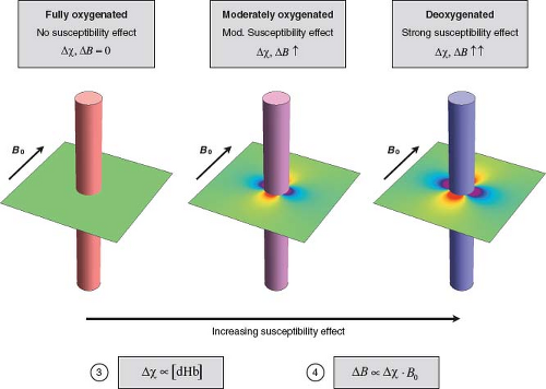 FIGURE 31.4 Deoxyhemoglobin (dHb) concentration modulates perivascular field perturbations. Colored cylinders represent capillaries or venules at different levels of oxygenation. The difference between intravascular and extravascular magnetic susceptibility (Δχ) increases in proportion to the concentration of intravascular paramagnetic dHb (Equation (3)). The compartmentalized differences in magnetic susceptibility generate perivascular magnetic field perturbations. The magnitude and distribution of the perivascular field varies with distance from the vessel, angular position around the vessel, and orientation of the vessel with respect to B0. The maximum perturbation at the vessel surface is a characteristic measure of its perturbing effect, denoted by ΔB. For illustrative purposes, all vessels are oriented perpendicular to B0, and the field is computed assuming that the cylinders are infinitely long. The perivascular field is illustrated in a plane perpendicular to the vessel. Areas of higher and lower field strength relative to the background field are indicated by shades of red and blue, respectively. The background field strength is indicated by pale green. The perivascular field has a dipolelike shape. Perivascular field perturbations increase in proportion to Δχ, and hence [dHb]. Left: Full oxygenation, indicated by the red cylinder. Since [dHb] = 0, the background field is unperturbed. Middle: Moderate oxygenation, indicated by the purple cylinder. Moderate [dHb] causes a moderate perivascular field perturbation. Right: Strong deoxygenation, indicated by the blue cylinder. High [dHb] causes a strong perivascular field perturbation. |
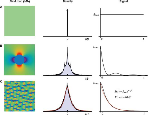 FIGURE 31.5 T2′ relaxation in the absence of spin diffusion: static dephasing. After RF excitation, each fixed spin precesses at a constant frequency proportional to the field strength at its locus (Larmor equation). Within a voxel, the distribution of frequencies is a scaled version of the distribution of field strengths. The dispersion of precession frequencies causes loss of spin phase coherence and, consequently, signal decay. The decay envelope is the Fourier transform of the frequency distribution and is not necessarily exponential. The Rows A, B, and C illustrate different spatial distributions of magnetic field (left), the associated distribution of magnetic field offsets (δB) (middle), and the resulting time course of the free induction decay (FID) or GRE signal decay (right), neglecting intrinsic T2 relaxation. A: Uniform field. Since all spins share the same precession frequency, they remain in phase and there is no signal decay. B: Dipolelike field distribution surrounding a single infinitely long cylinder perpendicular to B0, as discussed in Figure 31.4. Distribution of field offsets for spins outside cylinder shows a central peak due to peripheral spins at the background field strength, and two symmetrical side peaks, due to nearby spins in the dipolelike zones of higher and lower field strength, indicated by strong red and blue colors on the field map. The Fourier transform of this frequency distribution yields a nonexponential signal decay. C: Field distribution due to 100 randomly distributed infinite cylinders perpendicular to B0, for spins outside the cylinders. This arrangement models the random positions of microvessels within a voxel. (Additional randomization of the cylinder orientations provides a more realistic model, and decreases the magnitude of the effects, but the overall findings are unchanged [26].) The large number and random positions of cylinders within the voxel smoothes the distribution of field offsets, which closely approximates a Lorentzian distribution. The signal (black), therefore, closely approximates an exponential decay (red) (the Fourier transform of a Lorentzian distribution). (The early signal deviates from exponential decay, but later it closely approximates an exponential.) Monte Carlo modeling and experiments in model systems show that under conditions of static dephasing, the transverse relaxation rate increases in proportion to the characteristic field offset and vascular volume fraction, that is, in proportion to the tissue dHb content (Equations (3) and (4)): ΔR2′ = k · ΔB · V (see also Fig. 31.8). The constant k depends on the vessel geometry but is independent of vessel size. |
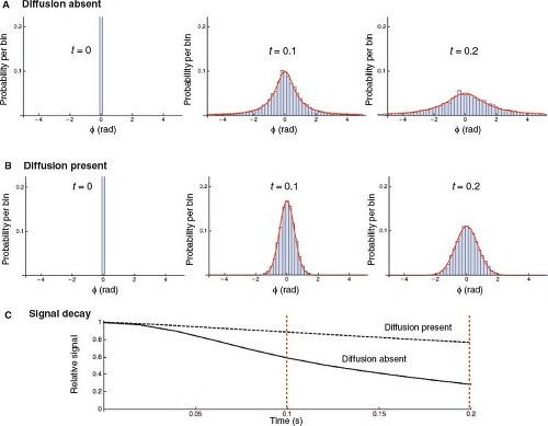 FIGURE 31.6 Spin diffusion decreases the R2′ relaxation rate. A,B: The progressive extravascular spin phase dispersion after radiofrequency excitation, without and with spin diffusion, in a model system simulating susceptibility-induced perivascular field perturbations. Results of Monte Carlo simulation using 10,000 spins randomly seeded within a plane perpendicular to 100 randomly positioned infinite cylinders perpendicular to B0, as shown in Figure 31.5C. Since motion parallel to the cylinders does not change the field, diffusion was modeled in the plane perpendicular to the cylinders. Spin phase distributions are shown at three discrete time points, t = 0, t = 0.1, t = 0.2 seconds. Histograms show probability per bin versus accumulated phase (φ) resulting from the simulation. Superimposed smooth red curves represent the best fit to model distributions. A: Static dephasing. At t = 0, all spins are in phase, with φ = 0. Over time, spin phases spread, always approximately conforming to a Lorentzian distribution, representing scaled versions of the Lorentzian magnetic field distribution shown in Figure 31.5C. B: Dephasing in the presence of spin diffusion. Random diffusive spin displacements cause motional averaging of spin phases. As a result, (1) the spin phase distributions are approximately Gaussian (normal distribution) instead of Lorentzian; and (2) at any given moment in time, the spin phase distribution is narrower compared with static dephasing (motional narrowing). C: FID or GRE signal decay in the absence (solid line) and presence (dashed line) of spin diffusion. Signal decay is approximately exponential in both cases. However, diffusion-induced motional narrowing reduces the rate of T2′ relaxation. (In both cases, the early signal deviates from exponential decay, but later it closely approximates an exponential.) The dashed red lines demarcate the two time points illustrated in panels A and B directly above. |
In turn, the capillary venous oxygenation determines the ratio of oxygenated to deoxygenated hemoglobin, while the concentration of deoxyhemoglobin [dHb] determines the magnetic susceptibility of the microvasculature. Assuming that the arterial blood is fully oxygenated, the fraction of hemoglobin that is deoxygenated is equal to the OEF. Therefore, the concentration of microvascular deoxyhemoglobin is
where [Hb] denotes the total blood hemoglobin concentration. Importantly, if neural activation were to increase CMRO2 and CBF by the same relative amount (i.e., percentage change), then the OEF, and hence deoxyhemoglobin concentration, would remain unchanged: there would be no consequent BOLD effect. Surprisingly, during neural activation, CBF increases
disproportionately to CMRO2, so OEF, and hence the microvascular deoxyhemoglobin concentration, falls: this key physiologic fact drives the existence of BOLD fMRI. Conversely, if CMRO2 were to increase disproportionately to CBF, then the OEF, and hence the deoxyhemoglobin concentration, would rise, resulting in a negative BOLD effect. These physiologic principles are summarized in Figure 31.3.
disproportionately to CMRO2, so OEF, and hence the microvascular deoxyhemoglobin concentration, falls: this key physiologic fact drives the existence of BOLD fMRI. Conversely, if CMRO2 were to increase disproportionately to CBF, then the OEF, and hence the deoxyhemoglobin concentration, would rise, resulting in a negative BOLD effect. These physiologic principles are summarized in Figure 31.3.
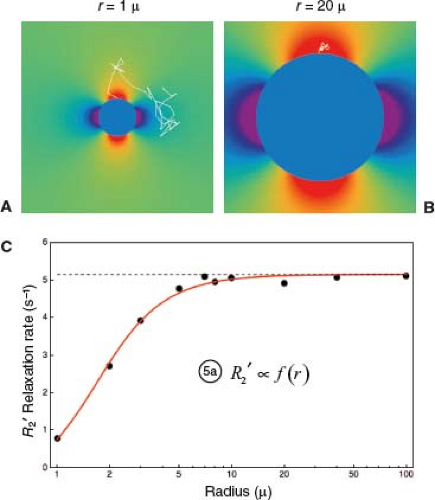 FIGURE 31.7 Spin diffusion causes R2′ to vary with vessel size. A: Diffusive motion around a small infinite cylindrical perturber of radius r = 1 μ, simulating a capillary (though smaller than most for illustrative purposes). Sample trajectory of a single spin, starting at the top surface, and followed over 4 ms in time steps of 0.1 ms, with a typical diffusion coefficient for brain water of D = 1 μ2/ms. Since the perivascular field falls off as (r/s)2 with perpendicular distance s from the centerline of the cylinder, and the radius is small, the field varies widely over the spatial scale of the diffusion trajectory: The spin samples a wide range of fields along its course, resulting in motional averaging of its phase history. As a result, diffusion strongly attenuates R2′ around small perturbers. B: As in A, but with r = 20 μ. With a large radius, the field varies little over the spatial scale of the diffusion trajectory: the spin samples a nearly constant field along its course, approximating static dephasing. As a result, diffusion does not significantly attenuate R2′ around larger perturbers. C: Monte Carlo simulation of FID or GRE T2′ relaxation due to infinite cylindrical perturbers of varying size, following methods similar to (26). For each cylinder size, the phase histories of 10,000 spins were computed as they diffused around randomly distributed cylinders oriented perpendicular to B0, at a fixed cylindrical volume fraction of 2%, with D = 1 μ2/ms and Δχ = 1.0 × 10⁻⁷ (in dimensionless cgs units). In each case, R2′ was computed by fitting an exponential to the computed signal decay. A log-linear plot of R2′ versus radius shows: (1) At larger radii, R2′ plateaus to a constant value because the diffusion effect is negligible in comparison with static dephasing (static dephasing regime), as illustrated in panel B. This result is consistent with the analytical model of (27), which predicts that R2′ is independent of cylinder radius for static dephasing (dashed black line). At smaller radii, R2′ declines because motional averaging progressively dominates static dephasing (motional narrowing regime), as illustrated in panel A. Equation (5) summarizes the vessel size dependence: R2′ is proportional to a factor that depends on vessel radius. The factor also depends on vascular volume fraction (CBV) and Δχ, but panel C illustrates the general shape of the size dependence. |
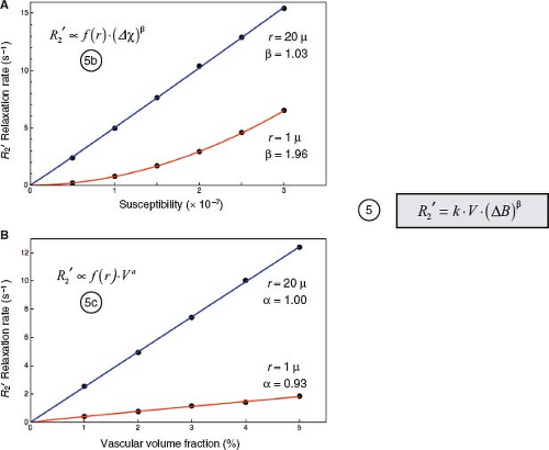 FIGURE 31.8 Dependence of R2′ on ΔB and CBV accounting for spin diffusion. Results of Monte Carlo simulations using the methods described in Figure 31.7C. Data points derive from simulations. Curves represent least-squares fit to power-law relationships, as indicated. A: R2′ versus Δχ, at a fixed vascular volume fraction of V = 2%. For large cylinders with r = 20 μ, where the static dephasing regime prevails, R2′ increases linearly with Δχ. For small cylinders with r = 1 μ, where the motional narrowing regime prevails, R2′ increases quadratically with Δχ. For intermediate cylinder sizes, R2′ ∝ Δχβ, where 1 < β < 2 (not illustrated). For a distribution of cylinder sizes that simulates cortical capillaries and venules, Monte Carlo simulations show a good fit with β = 1.5 (20,26) R2′ also depends on vessel size: at any given value of Δχ, R2′ is attenuated for r = 1 μ compared to r = 20 μ due to motional averaging, as illustrated in Figure 31.7. These results are summarized by Equation (5b). B: R2′ versus vascular volume fraction, V, at Δχ = 1.0 × 10⁻⁷ (cgs units). R2′increases linearly with V, independent of vessel size. Again, for any value of V, the vessel size dependence results in attenuation of R2′ for r = 1 μ (motional narrowing) compared with r = 20 μ (static dephasing). These results are summarized by Equation (5c). Noting that the strength of the field perturbation is proportional to Δχ · B0, the results in panel A would also apply by varying B0 instead of Δχ, so the Δχ dependence can be more generally replaced by a ΔB dependence. Finally, for a physiologic distribution of vessel sizes, the R2′dependence on V and ΔB can be summarized by Equation (5), where k depends on the vessel geometry and size distribution, and β ≈ 1.5. |
Deoxyhemoglobin Concentration Modulates Perivascular Magnetic Field Perturbations
Paramagnetic deoxyhemoglobin represents the interface between the physiologic and biophysical facets of BOLD signal formation. Specifically, the difference between intravascular and extravascular magnetic susceptibility, Δχ, is proportional to the concentration of intravascular deoxyhemoglobin:
In turn, Δχ induces local magnetic field perturbations around the vessels. The field perturbations decrease with distance from the vessel, vary with angular position around the vessel, and depend on the orientation of the vessel with respect to the direction of B0. However, the maximum perturbation at the vessel surface represents a characteristic measure of its perturbing effect, denoted here by ΔB. The magnitude of the perturbations scales in proportion to Δχ and B0:
Therefore, the magnetic field perturbations around capillaries and veins are stronger in proportion to their magnetic susceptibility, and hence deoxyhemoglobin concentration. These principles are summarized in Figure 31.4.
Perivascular Magnetic Field Perturbations Induce T2′ Relaxation
By the Larmor equation, perivascular magnetic field perturbations induce a proportional dispersion of precession frequencies. After radiofrequency (RF) excitation, the spins gradually lose phase coherence and the transverse magnetization decays approximately exponentially, characterized by the total transverse relaxation time T2*, or its reciprocal the total transverse
relaxation rate R*2. R*2 includes components due to intrinsic spin–spin interactions, R2, and to static field inhomogeneities, R2′, where R*2 = R2 + R2′. Since changes in vascular susceptibility alter R2′ but not R2, activation-induced changes in R*2 are reflected entirely by changes in R2′: ΔR*2 = ΔR2′, so that henceforth, we focus on R2′.
relaxation rate R*2. R*2 includes components due to intrinsic spin–spin interactions, R2, and to static field inhomogeneities, R2′, where R*2 = R2 + R2′. Since changes in vascular susceptibility alter R2′ but not R2, activation-induced changes in R*2 are reflected entirely by changes in R2′: ΔR*2 = ΔR2′, so that henceforth, we focus on R2′.
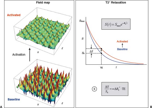 FIGURE 31.9 GRE BOLD signal change. A: Maps of magnetic field perturbations around randomly placed cylinders perpendicular to the magnetic field and the plot plane, simulating microvascular susceptibility effects, using the same configuration illustrated in Figure 31.5C. In the baseline condition, [dHb] is relatively high and perivascular field perturbations are strong. During activation, a disproportionate rise in CBF relative to CMRO2 and CBV decreases [dHb], so perivascular field perturbations are attenuated. B: Exponential decay of FID or GRE signal in the baseline (blue) and activated (red) conditions. Strong field perturbations in the baseline condition result in a relatively large R2′, hence rapid decay. Weaker field perturbations in the activated condition result in a comparatively small R2′, hence slower decay. At any given TE, activation causes the T2*-weighted signal to increase, representing the end result of the BOLD effect. The fractional change in GRE T2*-weighted signal is given by Equation (6). The BOLD signal is approximately proportional to the change in susceptibility-induced transverse relaxation rate and TE. |
T2′ Relaxation in the Absence of Spin Diffusion
In the absence of spin diffusion, all spins are fixed in position. The phase of any particular spin increases over time in proportion to the field strength at its fixed position. Therefore, at any moment in time, the distribution of spin phases is a scaled version of the distribution of field offsets, ΔB, relative to the unperturbed extravascular background field, or equivalently, the distribution of resonance frequency offsets, Δω = γ · ΔB, where Δω is the frequency offset in radians/s and γ is the gyromagnetic ratio of the proton. As a result, the signal-decay envelope is the Fourier transform of the frequency distribution. The distribution of field/frequency offsets is determined by the geometry and spatial distribution of the vessels. In general, transverse relaxation due to static dephasing in the setting of susceptibility-induced field perturbations is not exponential. However, analytical modeling (27), Monte Carlo modeling (26,28,29), and experiments in model systems (26,29) show that when the perturbers occupy a physiologically low fractional volume (i.e., CBV), the distribution of field/frequency offsets is approximately Lorentzian. Consequently, the signal decay envelope is approximately exponential (the Fourier transform of a Lorentzian distribution), and is well characterized by an exponential rate constant R2′. Under conditions of static dephasing, and considering only the effect of the extravascular spins (the vast majority), R2′ increases in proportion to the magnitude of the vascular field perturbations, ΔB, and their density (the vascular volume fraction, CBV, here denoted by V for brevity): R2′ = k · ΔB · V, where the constant of proportionality, k, depends on the vascular geometry, but is independent of the vessel size. In conjunction with Equations (3) and (4), we see that for conditions of static dephasing, R2′ is simply proportional to the tissue deoxyhemoglobin content, that is, the amount of deoxyhemoglobin per unit volume of tissue. The principles of static dephasing by vascular susceptibility effects are illustrated in Figure 31.5.
T2′ Relaxation in the Presence of Spin Diffusion
Diffusion of spins through the extravascular magnetic field perturbations adds nuance to the BOLD physics. Diffusion modifies the simple dependencies of R2′ on vessel size (independent), ΔB (linear), and V (linear) that occur with static dephasing.
Spin Diffusion: Motional Narrowing
In the presence of spin diffusion, the phase of any particular spin does not simply increase over time in proportion to a fixed frequency. Rather, the frequency of precession varies as the spin moves
randomly from place to place, experiencing slightly different fields at each moment in time. The net phase for any individual spin increases in proportion to the average of the phase shifts caused by the various fields that the spin encounters over the course of its random motion. This motional averaging has three consequences. First, in contrast to the static dephasing case, at any given moment in time, the distribution of spin phases is not a scaled version of the approximately Lorentzian distribution of magnetic field offsets, and the net signal is no longer the Fourier transform of the susceptibility-induced frequency distribution. Rather, as the spins randomly sample a large range of magnetic fields, the distribution of phases becomes approximately Gaussian, as with many other random processes (explained by the Central Limit Theorem in probability theory). Nevertheless, as in the static dephasing case, gradual spin dephasing still causes approximately exponential decay, which can be characterized by a relaxation rate R2′ (26,29). Second, different spins tend to experience similar average phase shifts because they sample a similar range of fields. At any moment in time, their net phase shifts are more alike than they would be in the static dephasing situation: that is, the distribution of spin phases throughout the sample (e.g., voxel) is narrower (motional narrowing). Finally, and most importantly for its effect on the BOLD signal, with less overall dephasing at any given time, the rate of relaxation induced by vascular susceptibility perturbations, R2′, is lower with diffusion than without it. The effects of motional narrowing on spin dephasing and T2′ relaxation are illustrated in Figure 31.6.
randomly from place to place, experiencing slightly different fields at each moment in time. The net phase for any individual spin increases in proportion to the average of the phase shifts caused by the various fields that the spin encounters over the course of its random motion. This motional averaging has three consequences. First, in contrast to the static dephasing case, at any given moment in time, the distribution of spin phases is not a scaled version of the approximately Lorentzian distribution of magnetic field offsets, and the net signal is no longer the Fourier transform of the susceptibility-induced frequency distribution. Rather, as the spins randomly sample a large range of magnetic fields, the distribution of phases becomes approximately Gaussian, as with many other random processes (explained by the Central Limit Theorem in probability theory). Nevertheless, as in the static dephasing case, gradual spin dephasing still causes approximately exponential decay, which can be characterized by a relaxation rate R2′ (26,29). Second, different spins tend to experience similar average phase shifts because they sample a similar range of fields. At any moment in time, their net phase shifts are more alike than they would be in the static dephasing situation: that is, the distribution of spin phases throughout the sample (e.g., voxel) is narrower (motional narrowing). Finally, and most importantly for its effect on the BOLD signal, with less overall dephasing at any given time, the rate of relaxation induced by vascular susceptibility perturbations, R2′, is lower with diffusion than without it. The effects of motional narrowing on spin dephasing and T2′ relaxation are illustrated in Figure 31.6.
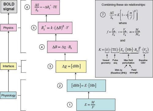 FIGURE 31.10 Synthesis of the Davis model for BOLD signal change, following (2,20,21). Six equations link activation-induced changes in CBF (F), CMRO2 (M), and CBV (V) to the fractional change in GRE T2*-weighted signal that constitutes the BOLD effect. The principles underlying these relationships are discussed in the text and illustrated in Figures 31.3–31.10, to which they are keyed. The magnetic susceptibility effect of paramagnetic deoxyhemoglobin (Equation (3)) is the interface between the physiologic (Equations (1) and (2)) and biophysical (Equations (4) to (6)) origins of the BOLD signal. Stepwise substitution of the model parameters, followed by algebraic rearrangement, leads to Equation (7), which expresses the BOLD signal as a function of dimensionless changes in CBF, CBV, and CMRO2. E = OEF. [Hb] = total intravascular hemoglobin concentration. F0, V0, and M0 denote baseline values. Fa, Va, and Ma denote activated values. The constant K has important implications for the BOLD signal. Its factors and significance are further discussed in the text. A typical value measured at 1.5 T is 8%. |
Spin Diffusion: Dependence of R2′ on Vessel Size
The effect of diffusion on R2′ is not an all-or-nothing phenomenon. Its impact depends on the balance between the tendency for static field perturbations to spread the spin phases and the tendency for diffusion to motionally narrow them. This balance plays out in a dependence of the BOLD signal on the radius of the perturbing vessels. The balance between static dephasing and motional narrowing can be described by characteristic time constants for the two processes. Static dephasing is characterized by the time required for a spin at the characteristic frequency offset Δω to undergo a characteristic phase shift of 1 radian: Δω · τsd = 1. Diffusion is characterized by the time required for a spin to sample a relatively large range of magnetic fields around the perturbers. Since the magnetic field produced by a cylindrical perturber of radius r falls off as (r/s)2 with perpendicular distance s from its centerline, the vessel radius is often taken as a characteristic average displacement for significant motional narrowing to occur. The time necessary for spins to diffuse an average distance r perpendicular to the vessel, τdiff, is given by the Einstein relation r2 = 4Dτdiff. If τdiff ≫ τsd, then the spins have abundant time to statically dephase before any motional averaging can occur, and static dephasing prevails, called the static dephasing regime. Conversely, if τdiff ≪ τsd, then significant motional narrowing occurs before the spins have time to undergo very much static dephasing, and motional narrowing prevails, called the motional narrowing regime. For example, for vessels modeled as infinitely long cylinders in random
orientations, the characteristic frequency perturbation is Δω = 4/3π · Δχ · γ · B0 (Δχ in dimensionless cgs units) (27). For blood at 60% oxygenation and a hematocrit of 40%, Δχ: 3.2 × 10⁻⁸ (27). Therefore, at 1.5 T, noting that the proton gyromagnetic ratio is γ ≈ 2.6 × 10⁸ rad/s/T, Δω = 53.9 rad/s and τsd = 18.6 ms. Using a typical diffusion constant of D = 1 μ2/ms for water in the brain, the characteristic diffusion time around a venule of radius 25μ is τdiff = 156 ms. Since τdiff ≫ τsd, spins operate well within the static dephasing regime around 25μ venules. Conversely, the characteristic diffusion time for a capillary of radius 3μ is τdiff = 2.25 ms. In this case, since τdiff ≪ τsd, spins operate well within the motional averaging regime around 3μ capillaries (Fig. 31.7A,B).
orientations, the characteristic frequency perturbation is Δω = 4/3π · Δχ · γ · B0 (Δχ in dimensionless cgs units) (27). For blood at 60% oxygenation and a hematocrit of 40%, Δχ: 3.2 × 10⁻⁸ (27). Therefore, at 1.5 T, noting that the proton gyromagnetic ratio is γ ≈ 2.6 × 10⁸ rad/s/T, Δω = 53.9 rad/s and τsd = 18.6 ms. Using a typical diffusion constant of D = 1 μ2/ms for water in the brain, the characteristic diffusion time around a venule of radius 25μ is τdiff = 156 ms. Since τdiff ≫ τsd, spins operate well within the static dephasing regime around 25μ venules. Conversely, the characteristic diffusion time for a capillary of radius 3μ is τdiff = 2.25 ms. In this case, since τdiff ≪ τsd, spins operate well within the motional averaging regime around 3μ capillaries (Fig. 31.7A,B).
More generally, when τsd and τdiff are comparable in scale, then neither the static dephasing nor the motional narrowing conditions dominate, and spins dephase in an intermediate regime. Therefore, R2′ varies continuously with the vessel radius. For large vessels, static dephasing dominates and R2′ plateaus at a large value. As the vessel size declines, so does R2′, because motional narrowing becomes progressively more significant. For any given values of Δχ and V, the dependence of R2′ on vessel radius can be generally summarized by
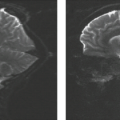
The vessel size dependence of R2′ has important implications for BOLD fMRI: the GRE BOLD effect is the strongest around larger venules and veins, and weaker around smaller capillaries. Therefore, at field strengths in the range of 1.5–3 T, the GRE BOLD effect tends to be somewhat biased away from capillaries in the activated cortex toward more peripheral draining venules and veins. “Anomalous” BOLD signals within larger cortical veins must sometimes be distinguished from true cortical activation.
Spin Diffusion: Dependence of R2′ on ΔB AND V
Spin diffusion also changes the simple linear dependence of R2′ on ΔB that characterizes the static dephasing regime. Interestingly, analytical models (30), Monte Carlo simulations (26,28), and experiments in model systems (26) show that when motional narrowing dominates, R2′ has a quadratic dependence on ΔB (Fig. 31.8A). When static dephasing dominates, R2′ maintains a linear dependence on ΔB (Fig. 31.8A). Generally, R2′ can be considered to hold a power law dependence on ΔB:
where β varies continuously between β = 1 for the static dephasing regime (e.g., around larger venules and veins) and β = 2 for the motional narrowing regime (e.g., around smaller capillaries). For a physiologic mixture of vessel calibers, Monte Carlo simulations indicate that β = 1.5 is a reasonable overall average value at field strengths of 1.5–3 T (20,26).
In contrast to the supralinear dependence of R2′ on ΔB, its dependence on the vascular volume fraction remains linear regardless of the vessel size (Fig. 31.8B) (26):
Spin Diffusion: The Net Effect on R2′
Combining Equations (5a) to (5c) yields the overall dependence of R2′ on the strength and volume fraction of the field perturbers, modified to include the net effects of spin diffusion:
where the constant of proportionality k depends on the geometry of the vasculature and the distribution of vessel sizes within the tissue.
Effect of Intravascular Spins on R2′
Thus far, the discussion has excluded the effects of intravascular spins, on the principle that their small volume fraction (a few percent) would cause them to have a minor effect on the total MR signal. However, Monte Carlo modeling and experiments in model systems have shown that this small volume fraction actually accounts for over 50% of the BOLD signal at field strengths in the range of 1.5–3 T, because the intravascular field perturbations around the red blood cells are much stronger than the extravascular field gradients around the vessels (31). The large intravascular field perturbations balance out the small vascular volume fraction, resulting in a surprisingly strong contribution from intravascular spins. However, it turns out that choosing β ≈ 1.5 fortuitously accounts for the effects of both diffusion and the intravascular spins (20,21,31).
The Davis Model for the Net GRE BOLD fMRI Signal
The GRE BOLD effect is measured by the relative change in T2*-weighted signal between the baseline and activation conditions:
where S0 and Sa are the signals in the baseline and activated conditions, respectively, and ΔR2′ is the associated change in transverse relaxation rate. Since the change in relaxation rate is small, the exponential can be replaced by its linear approximation:
 . Therefore, the BOLD signal is simply proportional to the activation-induced change in ΔR2′ (Fig. 31.9):
In turn, the preceding analysis connected CBF (F), blood volume (V), and oxygen metabolism (M) to the transverse relaxation rate, ΔR2′, induced by deoxyhemoglobin in the microvasculature, as embodied in Equations (1) to (5). Stepwise substitution of the model parameters into Equation (6), followed by simple algebraic rearrangement, yields a quantitative model for the magnitude of the BOLD signal change as a function of activation-induced changes in blood flow, blood volume, and oxygen metabolism, expressed entirely in terms of dimensionless parameters (illustrated in Fig. 31.10):
where f, n, and m denote activated blood flow, blood volume, and oxygen metabolism normalized to their baseline values:
and the constant K is
The constant K has two important interpretations (2). First, it represents a ceiling for the BOLD effect. The maximum possible BOLD signal change would occur if CBF increased so disproportionately to CMRO2 that it washed out all of the baseline deoxyhemoglobin and replaced it with oxyhemoglobin. Under this condition, ΔR2′ would decrease from its maximum possible value (occurring at baseline) to its minimum possible value of 0 (occurring during activation). This condition is approached as m/f → 0, with the physiologically reasonable assumption that n increases more slowly than m/f decreases. Equation (7) then shows that ΔS/S0 asymptotically approaches the maximum
possible value of K. Second, K is set by four main factors related to the underlying BOLD anatomy, physiology, and physics: (1) another constant, k, that is determined by the vessel geometry and the distribution of vessel sizes; (2) the NMR measurement time TE; (3) the strength of the perivascular field perturbations at baseline; and (4) the density of vascular field perturbers (i.e., CBV) at baseline, V0. The magnitude of the perivascular field perturbations is determined by the baseline intravascular deoxyhemoglobin concentration and the applied field strength B0. In turn, the baseline intravascular deoxyhemoglobin concentration is set by the baseline OEF and the total hemoglobin concentration.
possible value of K. Second, K is set by four main factors related to the underlying BOLD anatomy, physiology, and physics: (1) another constant, k, that is determined by the vessel geometry and the distribution of vessel sizes; (2) the NMR measurement time TE; (3) the strength of the perivascular field perturbations at baseline; and (4) the density of vascular field perturbers (i.e., CBV) at baseline, V0. The magnitude of the perivascular field perturbations is determined by the baseline intravascular deoxyhemoglobin concentration and the applied field strength B0. In turn, the baseline intravascular deoxyhemoglobin concentration is set by the baseline OEF and the total hemoglobin concentration.
Two additional relationships among the three physiologic variables, m, f, and v, allow the BOLD signal to be expressed as a function of a single physiologic parameter, such as the change in CBF. First, the fractional changes in CBF and CMRO2 are related through the ratio
 . For example, if neural activation causes a 30% increase in CBF and 10% increase in CMRO2, then n = 3. Typical measured values of n are in the range of 2 to 3 (21), while larger values have also been reported (6). For any given value of n, blood flow and oxygen metabolism are coupled by the relationship
 . Second, the relative changes in CBV and CBF are well described by an empirical power law relationship: v = fα, where α ≈ 0.4 (20,32). With these substitutions, Figure 31.11 shows the percent change in BOLD signal as a function of the percent change in CBF, for different values of n, using a typical empirical value of K = 8% at 1.5 T (20). For example, the model predicts that if neural activation causes a 50% increase in CBF, the BOLD signal change will be only in the range of 0.8% to 1.5% for n in the range of 2 to 3. As n → ∞, ΔS/S0 asymptotically approaches the maximum possible value of K = 8%. Finally, variations in K, n, and possibly β across brain regions, individuals, and time would lead to corresponding variations in the BOLD response. It is important to realize that these differences in the BOLD response may reflect differences in the physiology that couples neural activity to the BOLD signal, rather than true differences in underlying neural activity itself.
Related posts:
Stay updated, free articles. Join our Telegram channel

Full access? Get Clinical Tree


