FIGURE 3.1: Mean sac diameter. The gestational sac is measured in three planes with the calipers placed at the interface between the wall of the sac and the embryonic fluid. Notice that the sac wall is not incorporated in the measurement. The MSD is the average of the three measurements.

The gestational sac can often be confused with a pseudo-sac seen in ectopic pregnancy. To distinguish a true gestational sac, one must identify a double sac sign. This is a finding that is created by visualization of the two layers of the decidua parietalis. The deep layer of the decidua parietalis and early villi is more echogenic, and this can be seen as separated from the less echogenic layer of the superficial layer. Also, the intradecidual sign can be seen, where the sac is imbedded in the decidua rather than between two layers of the endometrium (Fig. 3.2).

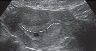
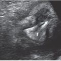
FIGURE 3.2: Characteristics of a gestational sac. In this image, the gestational sac is seen eccentrically located in the endometrial cavity. It is displaced inferiorly such that it is located in the decidua rather than the endometrial canal (line). The sac also has a hypoechoic rim around a hyperechoic sac wall.

As the first trimester advances, the reliability of the MSD in predicting menstrual age decreases. Between 2 and 14 mm, the MSD is quite precise in determination of age, but after a MSD of 14 mm, an embryo can be seen. Once an embryo is seen, the measurement of the crown rump length (CRL) can be obtained, and this is now more accurate in obtaining the true estimation of gestational age. The CRL is not the true measurement of the length of the fetus, as fetuses in early gestation have flexion. In truth, the CRL is the measurement of the longest straight line from the head of the fetus to the caudal end. Figure 3.3 depicts measurements of the CRL at different gestational ages. When obtaining the CRL, the sonologist should obtain at least three measurements and average the values to obtain the gestational age (see Table 1 in Appendix A1).

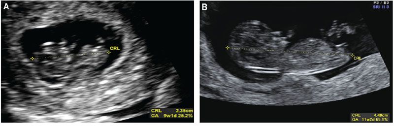
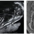
FIGURE 3.3: Crown rump length (CRL). A: The CRL is measured in a sagittal plane through the fetus. The image contains the head and body. Calipers are placed from the tip of the head to the edge of the caudal end. B: The CRL at later gestational ages (GA) allows for a clearer distinction of the fetal edges.

The accuracy of gestational age determination based on CRL is best in the middle of the first trimester. As the pregnancy advances, the CRL loses precision in gestational age determination.⁹ When examining pregnancies conceived through IVF, where the precise gestational age is known, from 7 to 11 weeks, the 95% confidence interval shows that the CRL is within 3 days of true gestational age. From 11 to 13 weeks, the 95% confidence interval is within 5 days.¹⁰ Hadlock et al.¹¹ showed that the variability in the CRL remained fairly constant from 2 mm to 12 cm, where the 95% confidence interval for gestational age was 8%. Therefore, if a pregnancy measured 8 weeks 0 days, the true gestational age was 8 weeks 0 days ± 0.64 weeks. If the pregnancy measured 12 weeks, the true gestational age was 12 ± 0.96 weeks. Variation in fetal growth in the late second and third trimesters is an expectation in any given population reflecting individual genetic determinants of growth, but deviation in fetal CRL size may be a predictor of growth pathology. Using pregnancies resulting from assisted reproductive technology, the FASTER trial showed that fetuses who measured small in the first trimester had a higher risk of being small for gestational age (SGA) later at birth.¹² Alternatively, fetuses measuring larger than expected by CRL in the first trimester also may be at risk for macrosomia at birth.¹³ Therefore, CRL is a useful tool not only for gestational dating, but it may also predict patients at risk for developing abnormalities in fetal growth as pregnancy advances.

Other measurements can be obtained in the first trimester that can help in the determination of gestational age. First trimester biparietal diameter (BPD) and abdominal circumference (AC) have been investigated by multiple authors. Two independent authors evaluated first trimester measurement of BPD and compared this with CRL between 7 and 13 weeks. Both showed that the CRL was superior to BPD in determining menstrual age.^14,15 This has come into question in a more recent analysis evaluating BPD and CRL in pregnancies conceived through IVF. In this study, the two measurements were similar in ability to predict gestational age, but the BPD had the advantage of having lower random measurement error.¹⁶ Another recent analysis showed similar findings when evaluating first trimester BPD, CRL, and AC. This analysis showed that both CRL and BPD were accurate in determining when a pregnancy will actually deliver, and both were superior to the fetal AC.¹⁷ Given the precision and ease of obtaining a first trimester CRL with high-resolution abdominal and vaginal ultrasonography, most practitioners utilize this measurement as the primary means of determining gestational age. However, in the event that CRL cannot be obtained because of fetal position, uterine anomalies, or maternal body habitus, first trimester use of the BPD could be an alternative measurement in determining gestational age.

First trimester ultrasound is the most accurate method of determining gestational age. The measurement of the gestational MSD between 2 and 14 mm, followed by CRL determination once a fetal pole is seen, will appropriately assign an estimated due date. Biological variability in the first trimester is present, but it is much smaller than later in gestation. Once a due date is determined from a precise first trimester ultrasound, this due date should not be changed later in gestation. If a future ultrasound shows significant deviation from the due date established by first trimester ultrasound, this identifies a fetus with abnormal growth. As detailed later in this chapter, these fetuses may be at risk for poor perinatal outcome and should have further evaluation.

SECOND AND THIRD TRIMESTER BIOMETRY

In order to calculate a second or third trimester gestational age, multiple structures should be evaluated with rigorous criteria, and those criteria will be discussed below.

Biparietal Diameter

The BPD was originally defined as the widest distance between the parietal eminences. However, this measurement is often more cephalad in location when compared with the thalami.¹⁸ Since standardization is the goal, the BPD is measured when certain landmarks are identified. The BPD can be measured in any plane that traverses the third ventricle and the thalami. By convention, the BPD is measured in a similar plane as the head circumference (HC), but since it is a single line that crosses through the thalamus, it can be measured in any plane. For the BPD to be accurate, the third ventricle and thalamus need to be identified and located centrally in the image. The calvarial walls should be symmetric, and the midline of the fetal brain should be equidistant from the parietal bones to ensure that an oblique measurement is not obtained as this will falsely increase the distance. The calipers are then placed on the outer edge of the proximal calvaria and measured to the inner edge of the distal calvaria (Fig. 3.4). With this measurement, the BPD is compared with a dataset to determine the percentile of the value, which can help to identify normal and abnormal growth (see Table 9 in Appendix A1).

FIGURE 3.4: Biparietal diameter (BPD). The BPD is taken in an axial plane with the midline perpendicular to the transducer. The thalamus (T) is seen in the center, and the cavum septum pellucidum (CSP) is noted in the front of the image. The calipers are placed from the outer edge of the proximal calvarium (C) to the inside edge of the distal calvarium.

Head Circumference

Unlike the BPD, the HC requires a specific plane for proper acquisition. To appropriately obtain the measurement, the proper plane needs to parallel the base of the skull, the transducer must be perpendicular to the parietal bones, and the image must transect the third ventricle and thalami. To ensure the correct plane of measurement, the cavum septum pallucidum (CSP) must be visualized as a box-like structure in the anterior portion of the fetal brain. The thalamus needs to be visualized around the third ventricle, and the cerebellum should not be in the image. If the cerebellum is seen, the image was obtained in an oblique plane, and this will increase the overall circumference measurement. Once the appropriate plane is obtained with identification of the appropriate structures, the HC is measured as an ellipse around the perimeter of the fetal skull. The HC does not include the skin edge; rather, an accurate HC traces around the calvarial margins. Ideally, the entire calvarium is visualized (Fig. 3.5). Often, images of the head shape appear abnormal, as in cases of breech presentation or fetal head molding. The fetal head is called dolichocephalic when transverse diameter appears flattened with the A-P diameter elongated. Conversely, the head is called brachycephalic when it appears more rounded than long. In both of these instances, the BPD may appear abnormal, but the overall size of the fetal head is within a normal range. The HC will not be altered by the relative shape of the head, and this provides an advantage over the BPD in determining whether a fetus has abnormal growth. Table 7 & 9 in Appendix A1 shows normal values for HC.

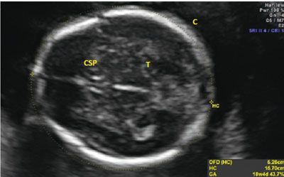
FIGURE 3.5: Head circumference (HC). The HC is taken in an axial plane. In the image, the landmarks of the thalamus (T) and cavum septum pellucidum (CSP) are visible. The midline is noted to be equidistant from both calvarial (C) edges. The HC is measured as the perimeter around the bone.

Abdominal Circumference

The AC is similar to the HC in that it requires a precise plane of obtainment in order to be accurate. Inclusive in the AC is the fetal liver, an organ that can be affected by pathological growth in that it will be small in instances of growth restriction because of glycogenolysis and large in instances of fetal macrosomia secondary to excessive glycogen storage. The appropriate AC incorporates the stomach, ribs, spine, and portal vein. The location of the confluence of the left portal vein and the right portal vein will create a “C-shape” in the fetal liver on ultrasound imaging, indicating an appropriate plane of obtainment. If the “C” is not seen in the fetal liver, either the transducer is too cephalad in the fetal abdomen or oblique to the correct plane. There should be one or two ribs seen in the image, but if the ribs are seen in cross-section with multiple segments visualized, the measurement will be falsely elevated. Figure 3.6 shows an appropriate image of the AC, including the stomach, portal vein, spine, and ribs. Tables 6 and 9 in Appendix A1 show measurements of the AC as gestational age progresses.

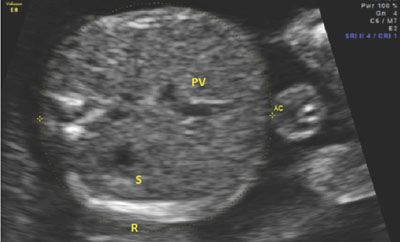
FIGURE 3.6: Abdominal circumference (AC). The AC is taken in an axial plain through the section of the abdomen containing the fetal liver. In this image, the liver is the proximal structure in the fetal abdomen. The portal vein (PV) can be seen curving away from the stomach (S). The PV makes a “C” shape, indicating that the image is taken appropriately. Additionally, the three bright spots on the left side of the image mark the spine. The rib (R) is seen at the bottom of the image of the abdomen. There is only one rib seen, indicating that the plane is not oblique to the fetal lie.

Femur Length

The femur is measured by aligning the transducer to the long axis of the femoral diaphysis. To measure the femur length (FL) correctly, the shaft should be aligned horizontally on the image. If the femur is not horizontal, shadowing from the edges of the bone will shorten the true length. Of note, ultrasound will detect only the ossified region of the femur, including the diaphysis and metaphysis. The cartilaginous regions are not well seen by ultrasound imaging. Once the entire length of the ossified bone is horizontal on the image, the calipers are placed on the central part of the femoral head and extended to the distal condyle. The calipers should be at the edge of the ossified site, between the bright bone and the dark cartilage. The correct measurement also does not incorporate the distal femoral point, as this is nonstandard and will incorrectly lengthen the measurement. Figure 3.7 depicts the proper measurement of the FL, and Tables 8 and 9 in Appendix A1 show the predicted gestational age for measured FL.

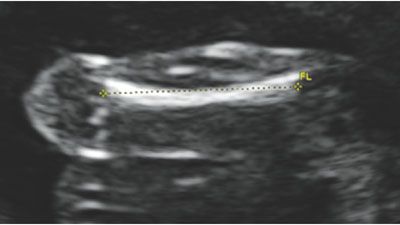
FIGURE 3.7: Femur length (FL). The femur length is measured with the longest portion of the bone perpendicular to the transducer. If the femur is not horizontal, shadowing from the ossified bone may shorten the length. The calipers are placed in the center of the femur and measured to the end of the bright edges, ensuring not to include the femoral tip.

ACCURACY IN MEASUREMENTS

Biparietal Diameter Accuracy

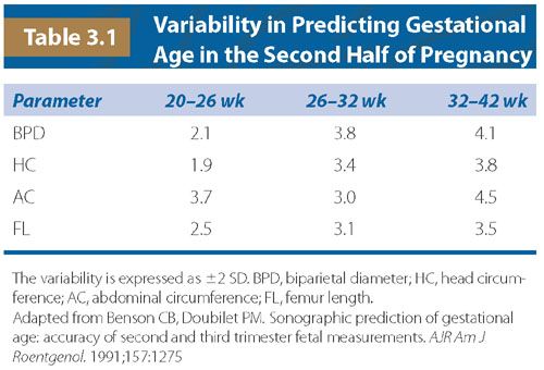
The BPD has been well studied in its accuracy in determining gestational age. Between 14 and 21 weeks, Hadlock et al.¹⁹ investigated 1,770 chromosomally normal fetuses, and they showed that the 95% confidence interval for measuring the BPD was within 1 week of the known gestational age. Other authors showed similar findings in accuracy between 14 and 20 weeks when looking at pregnancies dated either by known dates of conception or first trimester CRL.^20–22 In all of these studies, two standard deviations (SDs) for the accuracy of BPD in determining gestational age ranged between 0.92 and 1.02 weeks for gestational ages between 14 and 20 weeks. As gestational age advances, the variability of BPD measurement increases, diminishing the accuracy of gestational age determination. Benson and Doubilet²³ looked at pregnancies dated by early CRL, and they showed that the variability (±2 SD) in determining gestational age increased from 2.1 weeks at 20 to 26 weeks to 4.1 weeks from 32 to 42 weeks (Table 3.1). Similar to early CRL, BPD measurements are most accurate the earlier the study is performed, and as pregnancy progresses, deviation from normal will be more of a measure of abnormal growth rather than assigning gestational age.

As mentioned previously, the BPD can be significantly affected by the fetal head shape. In cases of breech presentation, uterine anomalies, fibroids, and multiple gestations, the fetal calvarium can be compressed so that the BPD is shortened or elongated relative to the true gestational age. The cephalic index (CI) is a ratio that assesses dolichocephaly and brachycephaly, and it is calculated from the BPD and the fronto-occipital diameter (FOD). This measurement is from the outside of the anterior portion of the fetal skull to the outside of the posterior calvarium. The CI is calculated as follows:

CI = (BPD/FOD) × 100

Hadlock et al. demonstrated that the CI remained relatively stable from 14 to 40 weeks, with a mean value of 78.3 and a SD of 4.4. In this study, CI measurements that were greater than 1 SD from the mean had BPD measurements that were inaccurate in determining gestational age. In such instances, the HC is a better measure as it is not as dependent upon head shape.²⁴

Head Circumference Accuracy

The HC is not dependent upon fetal head shape, and its measurement has also been shown to be an accurate predictor of gestational age. In fact, at less than 20 weeks, the HC may be more predictive of gestational age than BPD, as shown by Law and MacRae²⁵ Like the BPD, this measurement is accurate to within 1 week (±2 SD) of the gestational age when the precise due date is known. Like other measures in pregnancy, the best prediction of gestational age occurs with earlier measurement with error in accuracy increasing as gestational age advances.^19,21 In the third trimester, the inaccuracies of HC parallel that of BPD in gestational age determination with a margin of error of ±3.8 weeks (2 SD) after 32 weeks.²³

Abdominal Circumference Accuracy

The AC is the most difficult measure to obtain of all of the biometric assessments. Also, the AC contains the liver, which is subject to acute and subacute changes in metabolism by the fetus. In pathological states, it has been theorized that the liver size may shrink because of metabolic demands from nutrient deficiency. In instances of glucose excess, such as diabetes, the fetal liver should increase in size as glucose is stored in this organ. For these reasons, the AC would be expected to have the highest level of variability when predicting gestational age. This was observed by Benson and Doubilet²³ in their analysis, where they saw that the AC had the highest variability in predicting gestational age when compared with the other measures.

Femur Length Accuracy

With the ease of measuring the FL, this biometric parameter has been well studied in determining gestational age. Similar to other measures, the earlier the measurement is obtained, the more accurate the FL is in determining gestational age. As shown by Benson and Doubilet,²³ the FL has similar variability to other bony measures (e.g., BPD, HC) in the late second and third trimesters.

OTHER BIOMETRIC PARAMETERS

Multiple other structures have been investigated for determining gestational age. These include measurements of the binocular distance, clavicular length, ulna, tibia, radius, and foot. Similar to the other measurements, earlier assessment is most accurate. One structure that shows promise in accuracy is the transcerebellar diameter (TCD). This measurement can be obtained during evaluation of the posterior fossa. The best image is obtained by having the transducer perpendicular to the parietal bones, in a plane slightly diagonal to that used for the BPD. The optimal image has the CSP seen anteriorly and the cerebellum seen posteriorly. The calipers are placed on the outer edge of the cerebellum and measured to the opposite side (Fig. 3.8). Table 22 in Appendix A1 shows the measurements of the cerebellar length as gestational age advances.

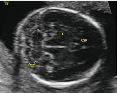
FIGURE 3.8: Cerebellar measurement. The cerebellum (Cereb) is measured from an axial plane in the fetal head. The plane is in the correct location when the cavum septum pellucidum (CSP) is located anteriorly with the thalamus (T) seen in the midline. The midline is equidistant from both calvarial edges.

The accuracy in gestational age determination for the TCD is quite high. Chavez et al. studied the TCD in the second and third trimesters in singleton, nonanomalous, well-dated pregnancies. Between 17 and 21 weeks, the TCD predicted gestational age accurately within 4 days. In fact, as pregnancy advanced, the TCD maintained a higher accuracy than any other biometric parameter. Between 29 and 36 weeks, the predicted age was within 5 days of the actual age, and at greater than 37 weeks, it was within 9 days.²⁶ However, measurement of the TCD may be challenging late in pregnancy. Fetal positioning and calcification of the skull can make visualization of cerebellar landmarks difficult. Unlike the BPD, HC, AC, and FL, the TCD is particularly important in determining gestational age at extremes of fetal growth. When evaluating pregnancies with good dating criteria, even in fetuses with growth restriction (estimated weight <10th percentile) and macrosomia (estimated weight >90th percentile), the TCD maintained accuracy in predicting gestational age.²⁷ Of note, like other measurements, chromosomally abnormal fetuses can have a TCD smaller than predicted,²⁸ which could further complicate assessment of gestational age. Despite this finding, clinicians are often challenged with patients presenting late in pregnancy with an uncertain gestational age. The TCD can be a measurement that will help in determining whether a fetus is measuring small or large for gestational age, as it seems to be less subject to variability when compared with other biometric parameters.

Although other long bone measurements do not provide any clear additional benefit for dating a pregnancy or for EFW calculation, in certain circumstances, they may be beneficial relative to bony abnormalities. Measurements for the humerus, radius, ulna, tibia, and fibula are captured in Table 17 in Appendix A1. The fetal foot length can be measured throughout gestation beginning as early as the end of the first trimester. The literature on newborn and fetal foot length has been summarized elsewhere,²⁹ and the foot length percentiles across gestation are shown in Table 18 in Appendix A1. In IUGR, Meirowitz and colleagues showed that 60% of fetuses have foot length measurements that are less than the 10th percentile. Thus, the foot length may not be sufficiently spared to provide clinical utility.³⁰

ESTIMATION OF FETAL WEIGHT

Up until this point, this chapter has focused on gestational age determination using ultrasound biometric parameters. This is crucial in determining the true due date and assigning an appropriate age to the pregnancy. Once the due date from early measurement has been established, it should not be altered later in pregnancy. In cases of deviation from the predicted gestational age, the fetus is demonstrating growth abnormalities—either in the case of excess fetal growth called macrosomia, or inhibited growth called FGR. Gestational age is not the only issue in assessing normal progression of a pregnancy; fetal weight is another key element in determining the status of growth.

Formulae

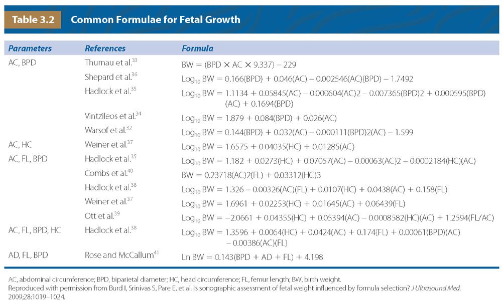
Shortly after the application of ultrasound to modern obstetrics, measurements of the fetus were evaluated in predicting birth weight (BW). One of the first publications showed that the AC alone was predictive of newborn weight with a moderate degree of accuracy if the AC was measured within 48 hours of delivery.³¹ With this observation, multiple other investigators started adding additional biometric parameters in an attempt to improve accuracy. Several authors added the BPD as the first measurement, and regression analysis was used to create standardized formulae for estimating fetal weight. Warsof et al.³² found that the addition of the BPD could improve accuracy with a SD of 106 g per kg if performed within 48 hours of delivery. Other investigators followed and generated other equations using the BPD and AC to estimate fetal weight.^33–36 Over time, FL was added to the equations in an attempt to improve prediction as the prior measurements did not take long bone growth into consideration. Additionally, BPD was recognized as being influenced by head shape, so HC was added to the equation in some instances, and replaced the BPD in others.^37–41 Table 3.2 shows some of the most commonly used equations in calculating an estimated fetal weight (EFW).

Accuracy of Specific Formulae

Numerous formulae exist for the estimation of fetal weight. Since none of the formulae has perfect accuracy, institutions may choose a particular formula as a standard or in specific scenarios. When looking at accuracy, investigators will assess bias (the systematic overprediction or underprediction of weight) and precision (random error). Systematic bias is often defined as the mean percentage error (MPE), where percentage error = 100 × (BW − EFW) / BW, and the MPE is the mean of per cent errors in a given population. Random error is the SD of the MPE. This method has been used to compare the accuracies of different formulae, and it is one tool that can help to determine which formula may be best. Of note, if an estimate of weight is calculated and the fetus progresses beyond one week from the measures, the EFW would be expected to be incorrect because of ongoing fetal growth. Additionally, maternal body habitus has a significant effect on accuracy, where the MPE in women with a body mass index (BMI) > 30 is almost double that in women with a BMI < 25.⁴² Therefore, appropriate comparisons can be made only if the EFW is made close to the time of delivery in a population where visualization of the fetus is possible.

Multiple factors can play a part in EFW accuracy, but how important is the specific formula used? When looking at each formula, using the same measurements from an individual fetus can provide considerable differences in values. Anderson et al. evaluated 12 different formulae for accuracy in population data from 1991 and 2000. They compared intraobserver and interobserver variability, and also looked at different formulae in the accuracy of predicting BW. They found that observer error (that obtained from multiple measures or from multiple sonologists on the same fetus) provided far less error than the use of different formulae. In fact, only six formulae were able to provide an MPE within 7%.⁴³ Edwards et al.⁴⁴ found that Hadlock³⁵ and Shepard¹⁸ provided more accurate results than other formulae. A systematic review of articles comparing EFW formulae was performed in an attempt to determine accuracy. In this analysis, the formulae by Hadlock et al. using BPD, HC, AC, and FL^35,38 seemed to provide the most consistent MPEs when used on various populations with the same amount of precision as other formulae. However, all formulae presented a fairly wide MPE and SD, and the authors conclude that no particular formula is ideal.⁴⁵ Other authors found that between 2,500 and 3,999 g, the Schild et al.⁴⁶ formula is the most accurate in determining weight (EFW = − 4,035.275 + 1.143 BPD³ + 1,159.878 AC¹/² + 10.079 FL³ − 81.277 × FL²). However, in this study most formulae performed similarly, and the MPE was still around 7% for the best ones.⁴⁷ Another group looked at multiple formulae and determined that for a general population, the formula by Hadlock [Log₁₀ EFW = 1.335 − 0.0034(AC)(FL) + 0.0316(BPD) + 0.0457(AC) + 0.1623(FL)]³⁸ had the lowest MPE with a sensitivity of 72% to 100% and specificity of 41% to 88% for detecting FGR.⁴⁸ The above studies have consistent findings, and Hadlock’s formula may be more accurate than others in determining fetal weight, but most formulae are similar and even the best do not have an MPE <5%. Further studies may help to identify the optimal formula given a specific population.

Accuracy at Extremes of Measurement

EFW accuracy can be affected by multiple factors, and one of the most significant factors influencing inaccuracies is the fetus demonstrating abnormal growth. In the EFW formulae, FL, BPD, and HC are all measures of bony structures. The AC is the only measurement incorporating soft tissue, as it encompasses the outer perimeter of the abdomen, which includes the liver and subcutaneous tissue. Investigators have argued that formulae based on bone structures may be less accurate with abnormal growth. In growth restriction, nutrient deficiency may lead to a more pronounced decline in muscle and fat cell growth compared with bone growth. In macrosomia, subcutaneous tissues would be expected to be increased, and the current formulae could be particularly inaccurate owing to the lack of accounting for this tissue development.

Multiple studies have been published addressing the issue of accuracy in EFW determination at extremes of newborn weight. Dudley showed that regardless of EFW formula, all methods showed wide variation in accuracy when the BW was less than 1,500 g. Additionally, for macrosomic newborns, the formulae were also more inaccurate with a tendency to underestimate weight.⁴⁵ Ben-Haroush et al. studied 840 pregnancies that were induced for various reasons and had an ultrasound EFW from 1 to 3 days prior to delivery. In this cohort, ultrasound EFW underestimated suspected macrosomic fetuses by a mean of 110 g and overestimated suspected growth-restricted fetuses by 113 g.⁴⁹ The same group also looked at 26 different formulae and found that models that incorporated 3 or 4 biometric indices were more accurate than those that only used 1 to 2. All models confirmed previous findings that the accuracy decreased at the extremes of newborn weight, where they overestimated low BW and underestimated large BW.⁵⁰ Regardless of the formula used, inaccuracy in EFW calculation exists when fetuses are small or large.

EFW is crucial in pregnancy management, where pregnancies identified as growth restricted will have increased surveillance and earlier delivery. Pregnancies identified as macrosomic will have changes in delivery planning in regard to route and timing. Clearly, improving accuracy at extremes of fetal weight will better guide the clinician in management of a specific pregnancy. As mentioned above, certain EFW models may be superior to others given a small or large fetus. In one study, when evaluating pregnancies with BW <2,500 g, Hadlock’s formulae (Log₁₀ EFW = 1.3596 − 0.00386 AC × FL + 0.0064 HC + 0.00061 BPD × AC + 0.0424 AC + 0.174 FL) and (Log₁₀ EFW = 1.335 − 0.0034 AC × FL + 0.0316 BPD + 0.0457 AC + 0.1623 FL)³⁸ were the most accurate when compared with 11 other formulae in predicting EFW.⁴⁷ In a different study, for fetuses expected to be <10th percentile, investigators found that symmetric (all measures small) versus asymmetric (AC and FL smaller than head measurements) growth restriction also affected accuracy in EFW. For symmetrically grown fetuses, Hadlock formulae incorporating three or more measures were the most accurate in determining weight. However, in asymmetric fetuses, the Hadlock formula with only two measures that excluded FL was more accurate.⁵¹ Studies investigating small fetuses show that Hadlock’s formulae have the highest degree of accuracy, but in the macrosomic fetus, other formulae could provide more appropriate EFWs. When comparing 36 commonly used formulae for EFW on 350 singleton fetuses with BW >4,000 g, Hoopmann et al. showed that Hart’s formula (e^7.6377445039 + 0.0002951035 × Maternal Weight + 0.0003949464 × HC + 0.0005241529 × AC + 0.0048698624 × FL [g, mm])⁵² had the lowest MPE and the highest detection rate for macrosomic fetuses. This method also showed that 96% of fetuses fell within 10% of the EFW.⁵³

Certain formulae may be more accurate than others at the extremes of fetal weight, but it may be that customizing a calculation provides the most accuracy. In a Chinese study of 1,034 patients, comparing 25 existing models failed to demonstrate a superior formula for EFW calculation. In this group, they created a regional-specific EFW model that could be used on the whole population. When the model predicted fetuses >90th percentile or <10th percentile, two different formulae were used: one for small fetuses and one for large fetuses. Using this method, they were able to more accurately predict fetal weight in growth-restricted and macrosomic fetuses.⁵⁴ Estimates of fetal soft tissue mass have been attempted to be measured through three-dimensional (3D) fractional thigh volume, which is an attractive addition to EFW formulae for the accurate prediction of weight in fetuses at the extremes of gestational age.⁵⁵ In one study, it showed superiority over conventional formulae for predicting actual BW in diabetic pregnancies.⁵⁶

Accuracy Conclusions

The literature has yet to declare a clear superior formula in the prediction of fetal and newborn weight. Factors affecting EFW include maternal body habitus, formula used, individual variability of the measures taken, and extremes of fetal weight. Although new models incorporating 3D technology have promise because they can evaluate fetal soft tissue mass, their clinical utility has not yet been adequately studied, and they have not yet entered into common practice. It seems that formulae involving three to four measures are more accurate than those involving one to two except in asymmetrically growth-restricted fetuses. It is recommended that each institution use a consistent formula for assigning an EFW rather than altering the formula for each patient. Universal application would lead to less confusion and more uniform care.

GROWTH CURVES

A growth curve is a graphic model of data that identifies the normal range of growth given a specific gestational age. Outliers are classified as too large or too small. Usually, a fetus measuring greater than the 90th percentile is defined as large for gestational age (LGA), while a fetus measuring less than the 10th percentile is defined as SGA. SGA was originally defined in 1967 by neonatologists to categorize a newborn with a birth weight of <10th percentile.⁵⁷ Over time, SGA was adopted by obstetricians to broadly classify the undergrown fetus regardless of etiology. The correct classification of fetuses as large or small is needed to accurately identify those fetuses that are at risk for poor perinatal outcome. An ideal standard would therefore allow a clinician to appropriately identify a pregnancy as high risk, and a good growth curve is the screening tool that would inform a clinician that increased surveillance is necessary.

Population-Specific Growth Curves

Normal neonatal birth weight differs depending upon the population studied. Race and ethnicity are key factors in determining normal weight, where black infants have lower mean birth weights than white infants.^58,59 Chinese neonates are lighter than newborns in the United States,⁶⁰ and Asian newborns are smaller than European newborns.⁶¹ It is not surprising that newborns of different races and different locations across the globe have different birth weights, but even when looking at birth weight ranges in Europe, regional differences exist. Knowing that differences exist is one thing, but does a birth weight in one region portend a different prognosis than the same birth weight in another region? One study by Graafmans and coworkers tried to answer this question. They compared the modal birth weights in specific countries, and they investigated their relationship to country-specific mortality curves. They found that shifts in the modal birth weight values paralleled the shift in the perinatal mortality curve. For example, Scotland has a modal birth weight of 3,446 g, with the lowest perinatal mortality found at 3,888 g. Norway has a heavier modal birth weight of 3,622 g, and the perinatal mortality nadirs at 4,305 g.⁶² This shows that perinatal outcome related to birth weight is regionally specific, and each population has an “ideal birth weight.” Many countries and institutions have created locally derived birth weight standards, and the curves generated from the data sources identify newborns at risk for poor outcome based on the individualized regional population. This seems to be a good strategy to identify those pregnancies that should be truly classified as high risk.

Fetal versus Neonatal Growth Curves

Neonatal birth weight standards vary by population, and European standards have been created identifying different normal weights depending upon the country of birth.⁶³ In the United States, many birth weight curves have been created, with one of the first standards defined by Lula Lubchencko in Denver.⁶⁴ The use of this birth weight curve to the general population came into question as this standard reported the birth weights of newborns born at moderately high altitude, a known factor leading to smaller newborn size. This again emphasizes the importance of regional standards.

Questions began to arise about the validity of using a birth weight growth standard for in utero fetal weight standards as investigators realized that preterm birth was a pathological condition. In fact, at preterm gestational ages, the normal population is one in which the mother is still pregnant. As ultrasound technology improved, it was possible to estimate fetal weight using mathematical modeling by measuring certain fetal characteristics as described previously in this chapter. In 1991, Ott and coworkers compared birth weight percentile at various gestational ages as determined by an ultrasound-derived EFW curve versus a standard BW curve. When using the ultrasound fetal weight curve as the standard, they showed that the number of fetuses classified as IUGR (<10th percentile) decreased as gestational age advanced. If the birth weight curve was used to classify a newborn’s weight, the number of babies identified as IUGR remained static. This caused the authors to draw the conclusion that growth restriction and preterm birth are related.⁶⁵ Hadlock et al.⁶⁶ created the most commonly used fetal growth curve, which was based on cross-sectional analysis of ultrasound data. By comparing EFW curves and newborn BW curves, the questions to be answered are: (a) how do these curves differ, and (b) which growth standard better identifies fetuses at risk for adverse perinatal outcome?

To address the first question, Bernstein and colleagues created a regional ultrasound-derived EFW curve based on 1,331 normal pregnancies. They compared this curve with the same region’s BW data from 9,553 births at various gestational ages. The estimates for the 10th percentile at each gestational age were different for all ages except 37 and 38 weeks. In preterm gestations, less than 2% of EFWs fall below the 10th percentile on the birth weight standard. Conversely, more than 26% of ultrasound EFWs were greater than the 90th percentile on the birth weight standard.⁶⁷ In a French population, Salomon et al. compared an EFW standard with a birth weight standard created from 18,989 singleton, nonanomalous fetuses and neonates. The growth curves were significantly different, showing that the 50th percentile on the birth weight standard matched the 10th percentile on the estimated weight standard from 28 to 32 weeks’ gestation.⁶⁸ These two studies showed that a birth weight standard will underestimate the number of IUGR fetuses and overestimate the number of LGA fetuses when compared with a growth curve created by EFW.

If a growth curve derived from EFW differs from that derived from birth weight, which curve is better at predicting adverse pregnancy and neonatal outcome? A Canadian study compared the outcomes of 37,377 nonanomalous pregnancies between 25 and 40 weeks classified as IUGR on either a birth weight curve or Hadlock’s curve.⁶⁶ This study showed that infants classified as IUGR from a fetal weight standard were more likely to have preterm birth than those that were appropriately grown; however, if a fetus was classified as IUGR on the birth weight standard, there was no association with preterm birth. The fetal standard identified 90 fetuses that eventually experienced a perinatal death compared with 57 fetuses identified employing the birth weight standard.⁶⁹ By classifying a fetus as IUGR on a fetal weight standard, the ability to predict adverse pregnancy outcome is improved over that of using a birth weight standard. Like pregnancy outcomes, neonatal outcomes have also been investigated. Zaw et al. compared the outcomes of 1,267 newborns at less than 34 weeks and classified them as IUGR using either a Canadian birth weight curve or Hadlock’s curve. In this study, babies classified as IUGR on the fetal weight standard were more likely to have the neonatal outcomes of respiratory distress syndrome (RDS), bronchopulmonary dysplasia, intraventricular hemorrhage, and retinopathy of prematurity. If the birth weight curve was used, newborns classified as IUGR were more likely to have neonatal mortality, retinopathy of prematurity, and necrotizing enterocolitis.⁷⁰ The differences in predictive ability likely hinge on the fact that newborns identified as IUGR on the birth weight curve are the smallest infants using either schema.

Using a fetal standard on ongoing pregnancies will better identify fetuses at risk for pregnancy and perinatal morbidity, whereas using a birth weight standard will better identify those fetuses destined for neonatal mortality. It is the obligation of the obstetrician to identify a diseased state, where fetuses classified as high risk are at an increased probability of developing poor outcome. Mortality is only one factor when considering poor outcome; therefore, the authors suggest using a fetal weight standard, such as that created by Hadlock et al.,⁶⁶ when determining the percentile of a given EFW.

Individualized Growth Chart

Population growth curves can be generated using databases on either birth weight or EFW, but many have advocated that designing a regionally specific population curve is still not sensitive enough to appropriately identify those fetuses truly at risk for poor outcome. A baby born at 39 weeks weighing 3,000 g to parents both under 65 inches tall may not be at the same risk as a baby born at the same weight to parents who are above 70 inches tall. This has led some investigators to generate an individualized growth chart to more accurately identify the fetus at high risk.

Gardosi and coworkers have proposed a novel method for an individualized growth curve. This group observed that multiple factors influence a neonatal birth weight, including maternal height, weight in early pregnancy, parity, and ethnic group.⁷¹ Paternal height was also a minor variable that contributes to the infant’s weight.⁷² This group developed a software program to calculate a fetus’ “term optimal weight” using coefficients of adjustment for each of the aforementioned variables. These coefficients were generated from multivariate analysis of large, well-dated birth weight databases of term infants. The confidence interval for the optimal birth weight was determined by the coefficient of variation for the mean term birth weight of the population database. A growth curve for each gestational age is then created using a log polynomial equation described by Hadlock.⁷³ This novel approach allows for the generation of a growth curve that takes into consideration normal term birth weight and normal preterm EFW, while adjusting for factors specific to the parents of a fetus.

Using this methodology, Clausson and coworkers compared perinatal outcomes of infants identified as IUGR on a Swedish birth weight standard versus the individualized growth curve. Infants identified as appropriately grown for their individualized standard but <10th percentile on the birth weight standard were not at risk for poor outcome. Conversely, infants identified as appropriately grown by birth weight standards but <10th percentile on the customized curve had an increased odds ratio of having poor outcome.⁷⁴ The individualized growth curve had a better ability to predict perinatal outcomes such as stillbirth, neonatal death, and APGAR scores <4 at 5 minutes.⁷³ The findings from this study were confirmed in French, Spanish, and US populations.^75–77 Additionally, the methodology has been used to generate customized growth standards for multiple gestations. When comparing a growth curve customized for twins to a customized curve for singletons, the curve for twins was more accurate in predicting fetal demise.⁷⁸ From multiple studies, the individualized growth curve is superior to birth weight standards at identifying fetuses at risk for poor perinatal outcome.

The concept of an individualized growth chart that takes into consideration maternal characteristics, paternal factors, and fetal number and sex is an attractive one. However, few data are available comparing this model directly to a fetal growth curve. A large study by Hutcheon and collegues compared the individualized curve to a birth weight curve and Hadlock’s curve. When looking at 782,303 infants, compared with the birth weight standard, both the individualized standard and the fetal standard identified more fetuses as <10th percentile at preterm gestations. However, they identified a statistically similar number of patients as IUGR when compared with each other. Additionally, the study confirmed that the birth weight standard was inferior in predicting which fetuses will have stillbirth or neonatal death; however, the individualized curve was similar to the fetal standard in predicting these outcomes.⁷⁹ This study suggests that the true benefit of an individualized curve rests on establishing an in utero standard, and the effect of maternal and paternal characteristics is minimal. Further study is needed to confirm these findings; and until data are available, the use of a fetal growth curve, such as that provided by Hadlock et al.,⁶⁶ seems to provide as much accuracy as the individualized curve in identifying fetuses that are at high risk of poor perinatal outcome.

MAGNETIC RESONANCE IMAGING

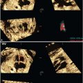
Ultrasound is the gold standard method for assessing fetal growth, but some authors have started using magnetic resonance imagining (MRI) as an adjunctive imaging modality in the assessment of at-risk fetuses. MRI has the advantage of a larger field of view, it is not affected by maternal body habitus or fetal position, and it has multiplanar and modal capabilities. One attractive feature of MRI is the ability to measure volume in 3D planes. In one of the first studies, Baker et al. measured fetal liver, placental, and brain volumes in 32 fetuses to see whether there was any association with newborn weight below the 10th percentile. Interestingly, the liver volume was <2.5th percentile in 10 of 11 fetuses who ultimately weighed less than the 10th percentile at birth. The placenta and brain did not show any reduction in measured volume compared with normally grown newborns.⁸⁰ Duncan et al. compared MRI with ultrasound in 74 fetuses, roughly half of which were growth restricted at birth. In this analysis, ultrasound fetal weight was superior to MRI in identifying fetuses that were measuring SGA. In contrast to the prior study, asymmetric IUGR fetuses (head size preserved) had reduced brain volume on MRI, suggesting that cerebral growth is still affected by growth restriction.⁸¹

Related posts:

Hydrops First Trimester Evaluation Neck Three-Dimensional Ultrasonography Multiple Gestation Normal Fetal Ultrasound Survey

Stay updated, free articles. Join our Telegram channel

Join