FIGURE 2.1: Scanners equipped with mechanical 3D transducers generate 3D volume datasets by automatically acquiring a sequence of 2D images through a ROI selected by the examiner. The images are reassembled into a final volume dataset that can be explored using postprocessing tools. The examiner can reslice the volume in virtually any plane, either to obtain rendered 3D images or to perform volumetric measurements. Most mechanical 3D transducers are also capable of 4DUS imaging, whereby multiple volume datasets are continuously acquired and quickly updated on the screen. With this technology, motion (temporal dimension) is added to the three spatial dimensions, allowing real-time visualization of 3D images. The primary limitation of 4DUS is that spatial resolution is often sacrificed at the expense of temporal resolution. (Reproduced with permission from Gonçalves LF, Joshi A, Mody S, et al. Volume US of the urinary tract in pediatric patients—a pilot study. Pediatr Radiol. 2011;41:1047–1056.)
Matrix Array Transducers
Matrix array transducers are full electronic transducers that consist of multiple (usually thousands) transducer elements arranged in a 2D matrix array configuration (Fig. 2.2). The face of the transducer has either a rectangular or a square shape. Matrix transducers can scan one line at a time (similar to mechanical probes described above), two planes simultaneously (orthogonal to each other or not), or an entire volume dataset by using multiple transducer elements simultaneously. Matrix array transducers are capable of real-time volumetric imaging, were originally designed for cardiac applications, but are now used in general and obstetrical imaging as well.15,19–23
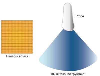
FIGURE 2.2: The “transducer face” diagram illustrates the typical configuration of a matrix array transducer, with thousands of elements arranged as a 2D matrix array, with each tiny square representing a single element. All elements, a portion of them, or two simultaneous lines can be activated simultaneously to produce real-time 3D images. The diagram “3D ultrasound pyramid” illustrates the pyramid of ultrasound that is emitted when all elements are fired simultaneously. The elements can also be fired in sequence, one line at a time, to produce volumetric data in a manner similar to the mechanical probe illustrated in Figure 2.1, just much faster.
Tips for Successful Volume Acquisition
Regardless of the choice of ultrasound equipment and type of volumetric probe, the reader is reminded that 3DUS is just an extension of 2DUS technology. Therefore, the same physics-related limitations apply. One cannot expect to compensate for poor 2DUS image quality caused by common problems such as patient obesity, oligohydramnios, and excessive bone shadowing by using 3DUS technology. Therefore, high-quality 2DUS imaging is a prerequisite for diagnostic 3DUS volume datasets.
Another issue that requires attention during volume acquisition is fetal movement. 3DUS technology has evolved over time to minimize movement-related artifacts by increasing acquisition speed while still maintaining acceptable image resolution, by the development of 4DUS technology for mechanical probes, and real-time volumetric imaging using matrix array probes. Still, excessive fetal movement can be a significant problem, not only because it can degrade image quality but also because it tends to generate artifacts that can affect image interpretation.24 Therefore, the sonographer has to scan smarter to compensate for fetal movement. Our anecdotal experience is that fetuses tend to move less during the early part of the exam, before the maternal abdomen is manipulated by the act of scanning. Our suggestion is that, if the purpose of the exam is the acquisition of volumetric data, the sonographer should begin the exam with a volumetric probe and attempt volume acquisition early. We also recommend careful attention to gentle scanning, avoiding excessive transducer movement and pressure, in an effort to prevent the initiation of movements by the fetus. In addition, once the 2DUS image is optimized and a good acoustic window to the structure of interest is present, volume acquisition should start without delay. The sonographer should avoid the trap of thinking that perfect 2D views (for example, a perfect facial profile or a perfect four-chamber view) are a prerequisite for high-quality 3DUS imaging. Although ideal, this is not necessary, since once a high-quality volume is acquired, these views can be obtained offline by image postprocessing. In fact, we propose that all that is needed for a good volume acquisition is a good acoustic window to the structure of interest in the absence of fetal movement. Therefore, if the target is the fetal face, all that is needed is that the face is oriented toward the transducer and that fluid is present between the face and the transducer. If the target is the fetal heart, similarly, all that is required is that the fetal chest faces the examiner and that no limbs are interposed between the fetal chest and the transducer. Again, the objective is an excellent acoustic window to the structure of interest, and not to pursue a perfect conventional 2DUS view prior to volume acquisition.
Postprocessing
Once the volume dataset is acquired, image postprocessing can take place at the scanner or at dedicated computer workstations. In the next few sections, we will review common approaches to explore 3DUS volume datasets.
Multiplanar Display
The multiplanar display is a simple but practical method to examine 3DUS volume datasets.5,25 This type of display typically shows three images, one representing the original plane of acquisition and another two orthogonal planes. A reference “dot” or “cross,” depending on the manufacturer, marks the intersection of the three orthogonal planes. As the user moves the reference “dot” or “cross” with a mouse or another electronic pointing device, any structure present in the volume dataset can be simultaneously displayed in three different planes. Figure 2.3 illustrates the basic principles of the multiplanar display method.
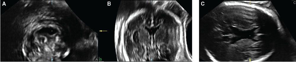
FIGURE 2.3: Multiplanar display of a volume dataset of the fetal brain acquired transabdominally using axial sections through the fetal head. The volume was manipulated so that the sagittal plane is shown in A, the coronal plane in B, and the original plane of acquisition, the axial plane, in C. The original plane of acquisition has the best resolution. The reference dot represents the intersection of the three orthogonal planes and, in this example, shows the typical imaging features of absence of the cavum septi pellucidi in the coronal (A), sagittal (B), and axial (C) planes.
Multiple Slice Imaging
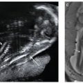
An alternative display method presents multiple slices of the volume dataset as a series of images in a single screen.26,27 This method, variously known as tomographic ultrasound imaging (TUI), multislice, or iSlice, depending on the manufacturer, permits simultaneous display of several consecutive planes of an organ or abnormality and may facilitate interpretation and/or teaching. Figure 2.4 shows features of tricuspid atresia with ventricular septal defect (VSD) using the TUI method.
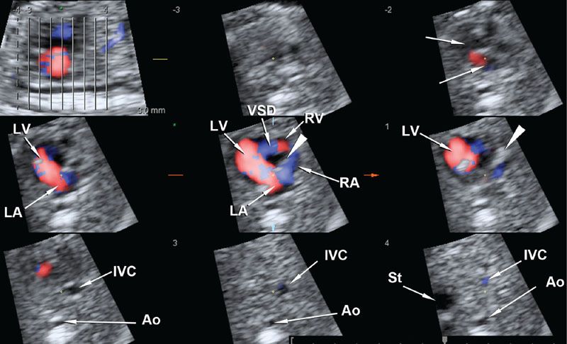
FIGURE 2.4: Multiple slice display of a volume dataset of the fetal heart acquired with color Doppler and spatiotemporal correlation (STIC). The left upper panel represents the scout sagittal view, with eight consecutive lines representing eight axial planes from the superior mediastinum to the upper abdomen shown in the next eight panels. The arrowhead points to the atretic tricuspid valve. Ao, abdominal aorta; IVC, inferior vena cava; VSD, ventricular septal defect; LV, left ventricle; RV, right ventricle; LA, left atrium; RA, right atrium.
3D Rendering
The term 3D rendering refers to the display method whereby a 3D object is displayed on a 2D screen using 3D photorealistic effects. The capability of presenting an image of the fetal face with surface rendering technology captured the attention of fetal imaging specialists and parents alike, and helped foster the initial interest in 3D obstetrical imaging.3,5,25,28
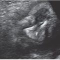
Surface Rendering: As the name implies, the surface rendering method is used when the intention is to display a 3D image of the surface of an object. This method works by displaying the first hyperechogenic voxel along the projection path of a volume dataset whose brightness is higher than a threshold determined by the user. The typical example is a rendered image of the fetal face (Fig. 2.5).
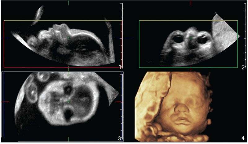
FIGURE 2.5: Multiplanar and volume rendered images of a normal fetal face acquired from a 2DUS facial profile view. Panels 1–3 show the sagittal, axial, and coronal orthogonal planes, respectively. A generous amount of amniotic fluid is interposed between the transducer and the skin surface of the fetal face. The boxes in panels 1–3, defined the ROI. The direction of view (or projection path) is determined by the user and, in this example, is given by the yellow line. Therefore, the first echo brighter than amniotic fluid (the threshold level) along the projection path is displayed as a pixel in panel 4 in order to form the rendered view of the fetal face.
Maximum Intensity Projection: In this rendering method, the voxel with the highest brightness signal along the projection path is displayed on the screen.4,25,29–32 In fetal imaging, this is typically used to display osseous structures, as illustrated in Figure 2.6.
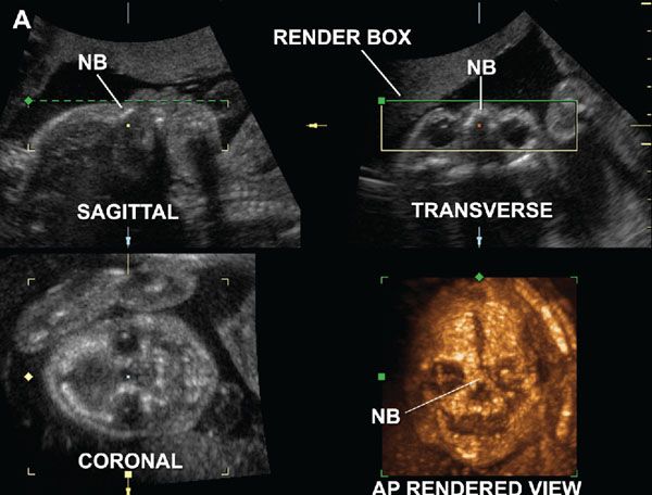
FIGURE 2.6: Normally developed nasal bones in a fetus with no abnormalities at 23 weeks of gestation. Multiplanar and anteroposterior rendered views of the fetal skull using the maximum intensity projection mode. The render box delimits the ROI, and the green line determines the direction of view for reconstruction of the 3D image. The paired nasal bones (NB) are visualized as a single structure fused in the midline. (Reproduced with permission from Gonçalves LF, Espinoza J, Lee W, et al. Phenotypic characteristics of absent and hypoplastic nasal bones in fetuses with Down syndrome: description by 3-dimensional ultrasonography and clinical significance. J Ultrasound Med. 2004;23(12):1619–1627.)
Minimum Intensity Projection: The minimum intensity projection method, as the name implies, displays the voxel with the lowest brightness signal along the projection path.25,33 This method is useful to display rendered images of fluid-filled structures. Figure 2.7 shows a rendered view of jejunal atresia displayed in the coronal plane.
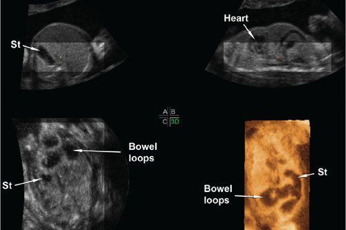
FIGURE 2.7: Multiplanar display of a volume dataset of a fetus with jejunal atresia. A–C show axial, sagittal, and coronal views of the fetal abdomen, respectively. The dilated loops of bowel are seen in the coronal plane. Panel 3D shows a rendered view of the abdomen using the minimum intensity projection mode. In this mode, the voxels with the lowest brightness signal along the projection path are preferentially displayed. In this case, a portion of the heart, the stomach (St), and the dilated bowel loops are the structures with the lowest brightness signal. They are simultaneously displayed in a single coronal view allowing the examiner to compare the relative positions of the bowel loops to the stomach, to determine that there are only a few dilated loops, and to note that the dilated bowel ends as a blind pouch in the left lower quadrant.
Average Intensity Projection: With average intensity projection, as the name implies, the average brightness of the voxels along the projection path are displayed as a pixel on a 2D screen. We use this method when we want to show rendered views of fetal limbs that simultaneously show the bones and soft tissues. Figure 2.8 shows the same fetal arm, forearm, and hand displayed using just the multiplanar display or volume contrast imaging (VCI, see detailed description below) with a slice thickness of 20 mm using the average intensity projection method.
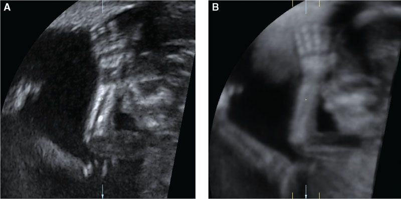
FIGURE 2.8: A: Single view of a fetal arm, forearm, and hand displayed using the multiplanar method. B: Volume contrast imaging (VCI) rendered view of the same arm using a 20-mm thick slab rendered using the average intensity projection method. Note that all fingers and the humerus are better seen on B when compared with A, with better demonstration of the soft tissues as well.
Inversion Mode: Inversion mode is a rendering method that inverts the grayscale of the voxels with the lowest brightness signal along the projection path. It is used for demonstration of fluid-filled structures.34–37 Figure 2.9 shows the same case of jejunal atresia previously seen using the minimum intensity project, now displayed using inversion mode. Although analogous, the inversion mode display allows further segmentation of the volume dataset and provides a better depiction of the anatomical relationships of the structures of interest.
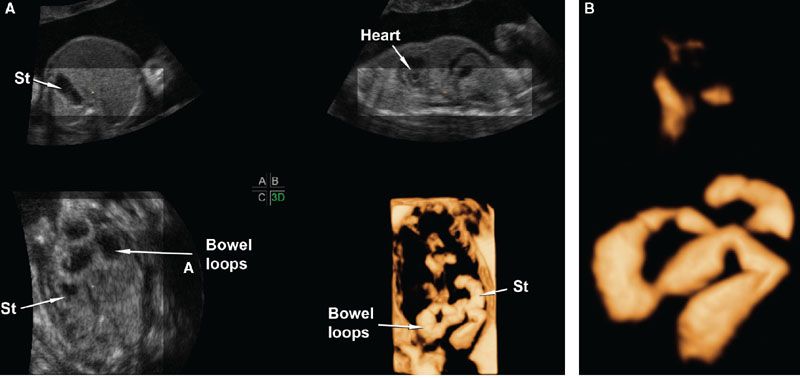
FIGURE 2.9: A: Multiplanar display of a volume dataset of a fetus with jejunal atresia. A–C show axial, sagittal, and coronal views, respectively, of the fetal abdomen. The dilated loops of bowel are seen in the coronal plane. Panel 3D shows a rendered view of the abdomen using the inversion mode method. The method is analogous to the minimum intensity projection mode, only that the voxels with the lowest brightness along the projection path are displayed with the grayscale inverted. B: In this image, further segmentation of the volume dataset was performed to display only the stomach (St), the duodenum, and the proximal jejunum. Part of the fetal heart is included only as a point of reference.
Volume Contrast Imaging: VCI is a rendering method that combines multiple consecutive frames together into a thick slab that can be displayed using any of the other rendering methods described above. Besides the example already provided in Figure 2.8, Figure 2.10 illustrates the improved tissue contrast resolution that can be obtained with this technology.
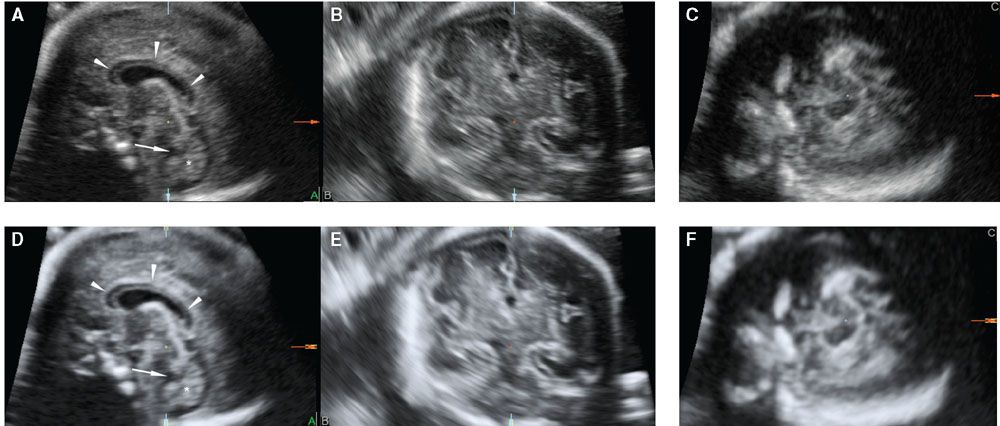
FIGURE 2.10: Multiplanar display of a volume dataset of the fetal brain obtained using a sagittal acquisition through the anterior fontanelle without (A–C) and with VCI (D–F). The corpus callosum (arrowheads), cisterna magna, fourth ventricle (arrow), and cerebellar vermis (star) are well depicted in both images; however, contrast resolution is better with VCI.
Postprocessing in the Ultrasound Equipment versus External PACS Systems and 3D Workstations: Image postprocessing is an integral part of volumetric imaging, and excellent results can only be expected once the examiner becomes comfortable with both volume acquisition and volume postprocessing. All ultrasound manufacturers provide volume manipulation and rendering capabilities directly in the ultrasound system. However, particularly when an examiner is learning 3DUS, volume manipulation and segmentation can be time consuming, and it may not be practical to tie the ultrasound equipment for this purpose (since it could otherwise be used to scan other patients).
The good news is that volume datasets can be manipulated in dedicated 3D workstations. Once exported, all capabilities available in the equipment are also available in 3D workstations. The problem that users face today is that ultrasound manufacturers use proprietary data formats that can only be opened using vendor-specific programs. Therefore, if the lab uses equipment from multiple manufacturers, the program interface to manipulate and segment volumes will be different, and programs from one manufacturer will not open volume datasets from the other, and vice versa. The hope of the ultrasound community is that full implementation of the 3DUS DICOM (Digital Imaging and Communications in Medicine) protocol will make 3DUS volumetric data available to all PACS systems with 3D manipulation and segmentation capabilities, regardless of the ultrasound system that generated the images, improving the learning process and workflow of 3DUS in clinical practice.38
FOUR-DIMENSIONAL ULTRASONOGRAPHY (4DUS)
4DUS is a term that describes the incorporation of a temporal component to the three spatial dimensions of a 3DUS volume dataset.8 Therefore, 4DUS allows the sequential display of multiple volumes as they are acquired and hence the capability of appreciating motion in volumetric imaging. This technology allows examiners to look not only at gross fetal movements (e.g., limbs) but also at more subtle fetal behavioral characteristics such as facial expressions (Fig. 2.11). Several investigators have applied this technology to study fetal behavioral states in utero, including the effect of adverse maternal and fetal disorders on expected behavioral patterns.39–46
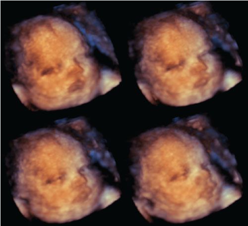
FIGURE 2.11: Series of rendered images of the face from a term fetus obtained with a real-time matrix array transducer. The images illustrate the capability of 4DUS to depict subtle changes of facial expression, such as eye opening.
4DUS of the Fetal Heart
Four-dimensional ultrasound of the fetal heart is possible by using spatiotemporal correlation (STIC) or real-time volumetric matrix array technology.7,11,13–15,47 STIC is a rendering algorithm that was developed specifically for fetal echocardiography applications. The algorithm essentially performs retrospective gating of the fetal heart rate to the acquired volume. The heart rate is calculated retrospectively from the raw volume dataset.7 The end result is that the multiple volumes of the fetal heart obtained in sequence through a single automated sweep of the fetal chest are reshuffled according to the phase of the cardiac cycle at which they were acquired. Provided that there is not excessive fetal motion during acquisition, excellent volume datasets of the fetal heart can be acquired, manipulated, and segmented using any of the display and rendering methods described in the “postprocessing” section above. Figure 2.12 shows the multiplanar display and rendered views of the atrioventricular valve orifices of a normal fetal heart acquired through a transverse sweep of the fetal chest.
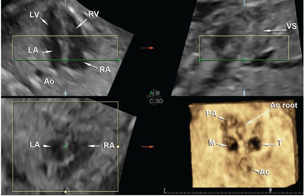
FIGURE 2.12: Volume dataset of the fetal heart acquired with STIC. A shows a four-chamber view of the fetal heart, B shows an orthogonal sagittal section through the ventricular septum (VS) displayed “en face,” and C shows a coronal section at the level of the atrioventricular (AV) valves. The rendered view of the AV valves is seen in panel 3D. Please note that the green line that determines the projection path is positioned within the atrial chambers (panels A and B) and, therefore, the rendered view is seen as if the examiner is looking at the AV valve orifices from the atrial chambers toward the ventricles. LV, left ventricle; LA, left atrium; RV, right ventricle; RA, right atrium; Ao, descending aorta; VS, ventricular septum; Ao root, Aortic root; PA, pulmonary artery; M, mitral valve orifice; T, tricuspid valve orifice.
FETAL ANATOMY BY VOLUMETRIC IMAGING WITH ABNORMAL EXAMPLES
In this section, we present a series of images that illustrate examples of both normal structures and pathology depicted by 3DUS and 4DUS, including the fetal heart.
Fetal Head
Figure 2.13 shows the sagittal corpus callosum reconstructed from a volume dataset originally acquired using a coronal sweep through the anterior fontanelle. This method is also suited for examination of the neonatal head using volumetric probes.48–50 Contrast the findings of this normal image with that of a fetus with absent cavum septi pellucidi shown in Figure 2.3. The same volume dataset is shown in Figure 2.14, now displayed using the multiplanar method with VCI set to a slice thickness of 3 mm to show the optic nerves and optic tracts at the level of the suprasellar cistern. Preliminary data show that the optic tracts and nerves can be successfully imaged using 3DUS rendering methods, and that optic tract measurements in the case of absent cavum septi pellucidi may help to identify those fetuses at high risk for septo-optic dysplasia.51
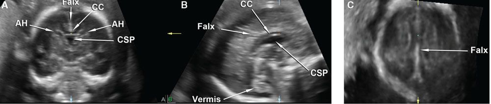
FIGURE 2.13: Multiplanar display of a volume dataset of the fetal head acquired using an automated coronal sweep through the anterior fontanelle. A shows the original coronal plane of acquisition, B shows the sagittal plane, and C shows the coronal plane. The reference dot is positioned at the anterior body of the corpus callosum, which is seen in its full length on the reconstructed sagittal plane. AH, anterior horns of the lateral ventricles; CC, corpus callosum; CSP, cavum septi pellucidi.
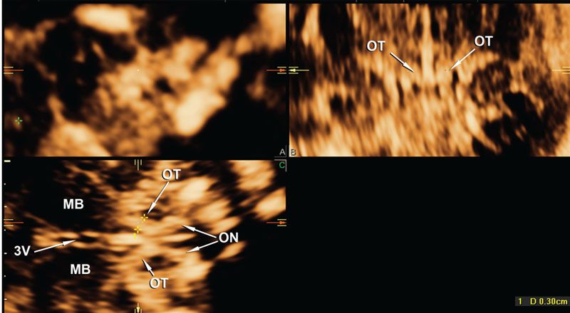
FIGURE 2.14: This image was produced from exactly the same volume dataset of the fetus with absent cavum septi pellucidi shown in Figure 2.3. The view is now magnified and displayed using VCI with a slice thickness of 3 mm. The sagittal, coronal, and axial orthogonal planes at the level of the suprasellar cistern are shown in panels A–C. The optic tracts and optic nerves can be clearly seen. OT, optic tracts; ON, optic nerves; MB, mid brain; 3V, third ventricle.
Fetal Face and Calvarium
3DUS is well suited for the evaluation of facial anomalies, with several studies documenting additional diagnostic information or better diagnostic accuracy when compared with 2DUS. 3DUS is useful for the evaluation of cranial sutures,4,52,53 facial bones,54–61 as well as cleft lip and palate.52,62–74
Figures 2.5, 2.6, and 2.11 illustrate the capabilities of 3DUS to depict normal facial structures and demonstrate subtle movements such as eye opening. The next few images illustrate the capabilities of 3DUS in the evaluation of selected craniofacial abnormalities. Figure 2.15 shows examples of hypoplastic and absent nasal bones in fetuses with trisomy 21.56,58 Figure 2.16 shows widened cranial sutures in a fetus with cleidocranial dysostosis. The same fetus had pseudoarthrosis of the right clavicle shown in Figure 2.17.
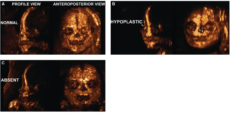
FIGURE 2.15: A: Normally developed nasal bones in a fetus with no abnormalities at 23 weeks of gestation. B: Delayed ossification or hypoplastic: Two small ossification centers can be seen away from the midline in the frontal projection and can be seen as a single hyperechogenic linear structure (owing to superimposition) in the sagittal projection. C: Absent nasal bones: No ossified nasal bones are present either in the frontal or in the sagittal projection. (Reproduced with permission from Gonçalves LF, Espinoza J, Lee W, et al. Phenotypic characteristics of absent and hypoplastic nasal bones in fetuses with Down syndrome: description by 3-dimensional ultrasonography and clinical significance. J Ultrasound Med. 2004;23[12]:1619–1627.)
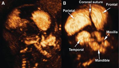
FIGURE 2.16: A: Three-dimensional (3D) rendering of the fetal skull at 18 + 3 weeks of gestation using the maximum intensity projection mode demonstrates widening of the coronal suture, absence of the squamous portion of the temporal bone, and absence of the nasal bones. B: Labeled 3D image of a normal fetal skull at 18 + 3 weeks (control). (Reproduced with permission from Soto E, Richani K, Gonçalves LF, et al. Three-dimensional ultrasound in the prenatal diagnosis of cleidocranial dysplasia associated with B-cell immunodeficiency. Ultrasound Obstet Gynecol. 2006;27[5]:574–579.)
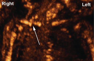
FIGURE 2.17: Three-dimensional rendering of the fetal shoulders using maximum intensity projection. The arrow points to the pseudoarthrosis of the right clavicle. (Reproduced with permission from Soto E, Richani K, Gonçalves LF, et al. Three-dimensional ultrasound in the prenatal diagnosis of cleidocranial dysplasia associated with B-cell immunodeficiency. Ultrasound Obstet Gynecol. 2006;27[5]:574–579.)
Evaluation of Orofacial Clefts
Volumetric imaging plays an important role in the evaluation of orofacial clefts and, therefore, deserves a separate discussion.
Orofacial clefts are common birth defects, being second in prevalence only to trisomy 21 according to a recent publication from the Centers of Disease Control of the United States.75 The most common types of orofacial clefts are isolated cleft lip, cleft lip with cleft palate, and isolated cleft palates. Median clefts are much less common and usually associated with chromosomal and structural brain anomalies. The adjusted United States prevalence of cleft lip with or without cleft palate was estimated as 1 in 1,574 live births, and that of isolated cleft palate as 1 in 940 live births. The prevalence in Asian and Native American populations is higher (as high as 1 in 500), whereas African-derived populations have a lower prevalence, estimated as 1 in 2,500. Approximately 70% of cases of cleft lip and palate, and 50% of cases of isolated cleft palate are nonsyndromic. The rest are associated with a wide range of malformation syndromes, chromosomal abnormalities and teratogen exposure. For a detailed review of the genetics and environmental factors associated with cleft lip and palate, the reader is referred to the excellent review article of Dixon et al.76
A diagram illustrating the anatomy of the palate is presented in Figure 2.18. Facial clefts can be unilateral or bilateral midline. When clefts involve only the lip, they are called isolated cleft lip or labioalveolar cleft. Clefts can extend to involve the primary palate (alveolus and premaxillary part of the maxilla, anterior to the incisive foramen) and/or the secondary palate (palatine process of the maxillary bones and palatine bone) (Fig. 2.19). In a large prospective ultrasound screening study from the Netherlands that included 35,000 low-risk and 2,800 high-risk patients, 40% of the clefts were clefts of the lip and palate, 29% were isolated cleft lip, and 27% were isolated cleft palate. Median and atypical clefts were rare and observed in only two fetuses. Sixty one per cent of the clefts were unilateral.
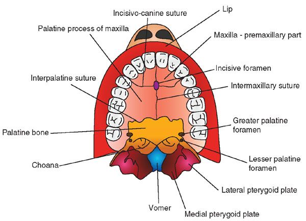
FIGURE 2.18: Normal palate anatomy.
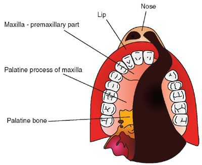
FIGURE 2.19: Diagram illustrating a unilateral cleft lip and palate involving the nose, lip, primary palate (anterior to the incisive foramen), and secondary palate.
Figure 2.20 shows the technique to properly acquire a volume dataset of the hard palate.74 Figure 2.21 shows how poor volume acquisition leads to shadowing artifact posterior to the tooth buds and, therefore, limited diagnostic value for the evaluation of the secondary palate.
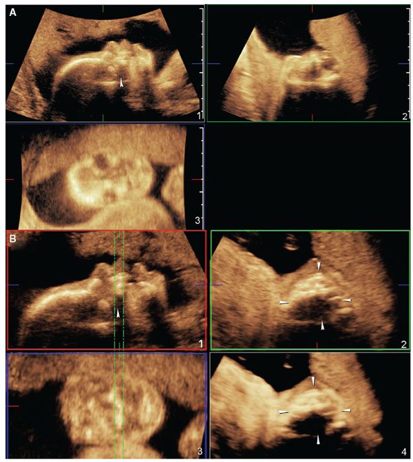
FIGURE 2.21: Contrast the volume acquisition in this figure with that in Figure 2.20. A: The facial profile is oriented in such a way that the hard palate is 0° with the transducer and therefore, a strong acoustic shadow is present posterior to the tooth buds (panel 1, arrowhead). B: The shadowing artifact is related exclusively to poor acquisition, and it cannot be corrected by postprocessing techniques. The same shadow seen in panel 1 (arrowhead) is seen posterior to the tooth buds in panel 2 and also in the maximum intensity projection rendered image displayed in panel 4. The anterior maxillary tooth buds can be well seen in panel 3.
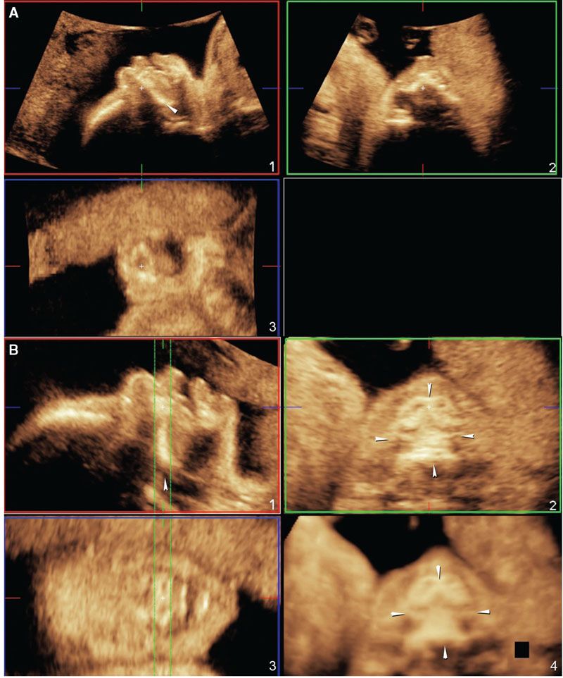
FIGURE 2.20: A: The ideal position of the fetal face for volume acquisition of the secondary palate. Note that the angle between the palate (arrowhead) and the transducer is approximately 45° (panel 1). B: Manipulation of the volume dataset to show the hard palate in its entirety. In panel 1, the volume is rotated around the z-axis so that the hard palate (arrowhead) is oriented at a 0° angle. In panel 2, the full extent of the hard palate can be seen in the axial plane (four arrowheads). Panel 3 shows the anterior maxillary tooth buds. Panel 4 shows a rendered view of the hard palate (four arrowheads) using the maximum intensity projection method.
Figure 2.22 shows an example of a rendered view of a unilateral cleft lip and palate with the 3D surface mode. Figures 2.23 and 2.24 show extension through the primary and secondary palates.
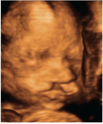
FIGURE 2.22: Three-dimensional surface rendered view of the fetal face. Unilateral cleft lip is seen on the left side.
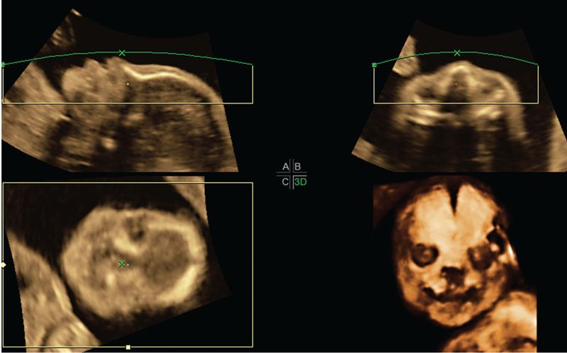
FIGURE 2.23: Multiplanar display and rendered views of the fetal face using the maximum intensity projection method to highlight the skull. A unilateral cleft lip can be seen going through the left alveolar ridge.
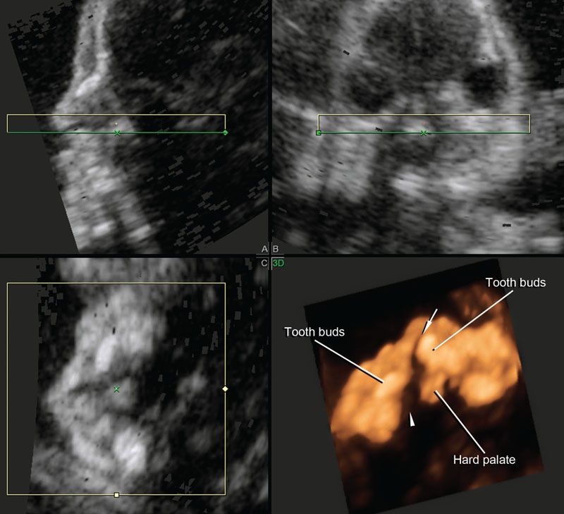
FIGURE 2.24: Reconstruction of the hard palate using the technique proposed by Platt et al.73 The rendered view using a combination of surface and maximum intensity projection modes shows that the unilateral cleft extends through the primary and secondary palates. Arrow, cleft of the primary palate; arrowhead, extension to the secondary palate.
Several investigators have compared the diagnostic performance of 2DUS versus 3DUS for correct classification of the type and extent of orofacial clefts. Collectively, the evidence supports 3DUS as a more accurate method, largely because of better characterization of the extent of hard palate involvement using multiplanar display and/or rendering techniques.64–67,69–71,73,74,77–85 In one of the comparative studies, Johnson et al.67 showed that 2DUS overestimated the severity of the defect in 41.9% (13/31) of the cases. Of interest, a recent study performed with 3DUS in the first trimester reported sensitivities of 100% and 86% for the diagnosis of clefts of the primary and secondary palate, with a 0.9% false-positive rate.86
Pitfalls
3DUS rendered images of the fetal face provide a visual realistic view of the defect that may help explain the abnormality to the parents and perhaps the surgeon who is involved in counseling. However, one must be careful in interpreting 3D rendered images alone and take into consideration the possibility of rendering artifacts or shadows that may create artificial clefts.87–89
In addition, ultrasound has traditionally not performed well for the evaluation of the soft palate, except for a recent series from Germany that reported on a new sign (“equal sign”) for evaluation of the soft palate and uvula. In that study, adequate visualization of the soft palate and uvula was possible in 85.3% and 90.7% of 667 consecutively examined fetuses.90 Magnetic resonance imaging (MRI) is a good adjunctive imaging modality for visualization of the soft palate.91–93
Fetal Spine
3DUS is a useful adjunct to 2DUS for the examination of the fetal spine. Besides its role in the characterization of segmentation abnormalities and abnormal curvature of the spine, 3DUS has proven accurate with one vertebral segment to determine the level of the defect in cases of spinal dysraphism (Fig. 2.25).30–32,94–99
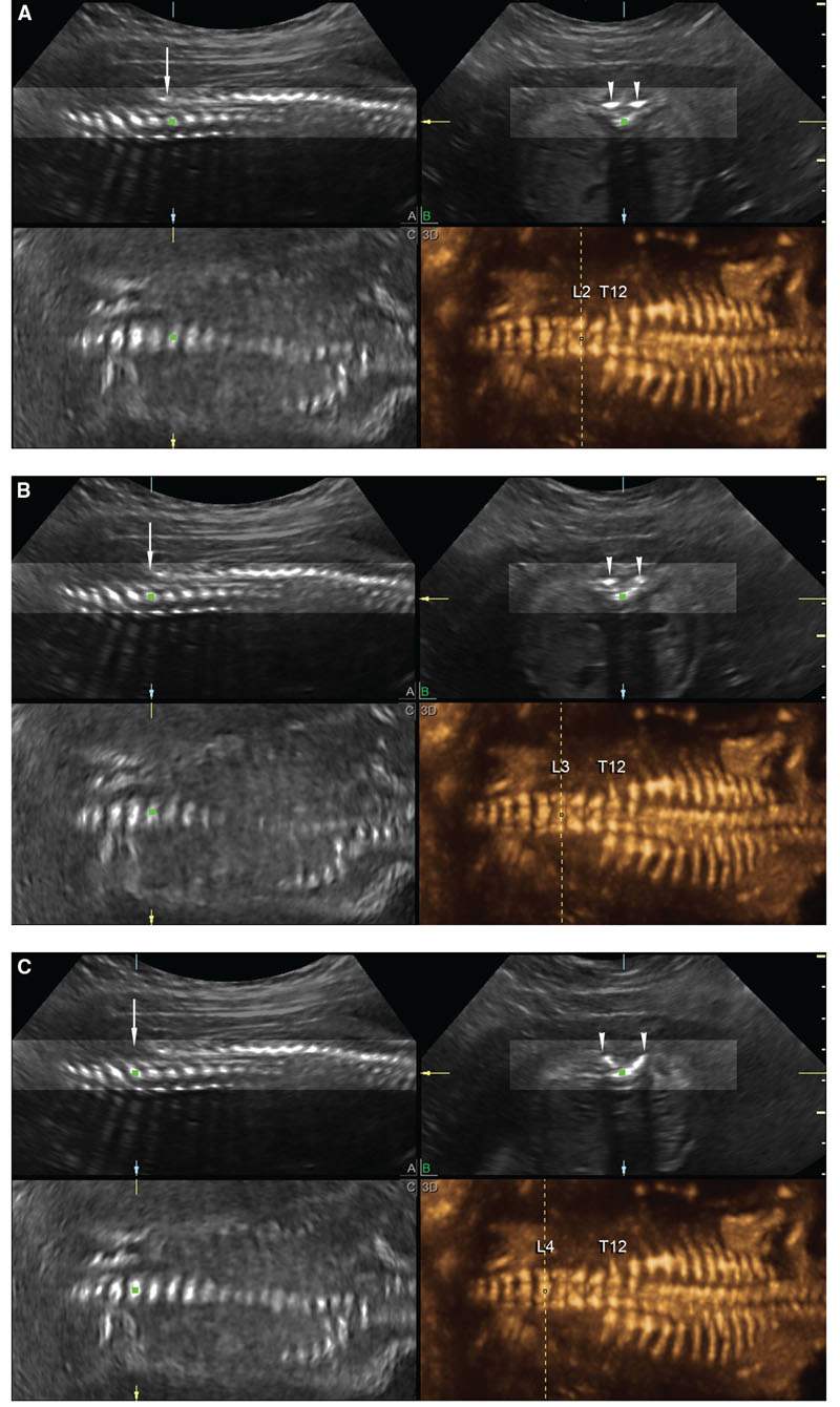
FIGURE 2.25: Multiplanar display (A is sagittal; B, transverse; and C, coronal) and rendered views (panel 3D) of the fetal spine in a fetus with open spinal dysraphism and a mild scoliosis. A: A vertical dashed line corresponds to the level at which the three planes intersect at L2. The posterior laminae of the spine are closed at this level (arrowheads in B). B:. The vertical dashed line is at the level of L3; the posterior elements begin to splay at this level (arrowheads in B). C: The posterior elements are clearly splayed at the level of L4 (arrowheads in B).
Skeletal Dysplasias
The ability of 3DUS to obtain rendered images of the fetal skeleton makes it a useful adjunctive modality in the diagnostic workup of skeletal dysplasias (see Figs. 2.16 and 2.17) and musculoskeletal disorders (Fig. 2.26). Several case reports have been published highlighting potential benefits of 3DUS for the visualization of specific features of skeletal abnormalities, for example, enhanced visualization of femoral and tibial bowing in a case of platyspondylic lethal chondrodysplasia, hypoplastic scapulae in campomelic dysplasia, improved characterization of frontal bossing in thanatophoric dysplasia, demonstration of caudal narrowing of the interpedicular distance of the lumbar spine in achondroplasia, improved visualization of epiphyseal stippling in chondrodysplasia punctata, better characterization of the abnormal spine and ribs in Jarcho-Levin syndrome, visualization of genu recurvatum in Larsen syndrome, and pseudoarthrosis of the clavicle in cleidocranial dysostosis.100–108 Few studies, however, have directly compared 3DUS versus 2DUS for the prenatal diagnosis of skeletal dysplasias, with the exception of the study of Ruano et al.,109 who showed higher visualization rates for skeletal structures by 3DUS (77.1%) when compared with 2DUS (51.4%), but lower than helical CT reconstructions (94.1%).
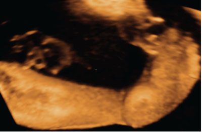
FIGURE 2.26: Three-dimensional rendered view of the fetal leg and feet showing clubfoot.
Congenital Heart Disease
Accurate prenatal diagnosis of congenital heart disease (CHD) is an important goal of prenatal care. Besides affording the parents appropriate and timely counseling, advanced knowledge of ductal-dependent anomalies allows planned delivery at institutions equipped to handle such cases, both from the medical and from the surgical standpoints. Indeed, prenatal diagnosis of CHD, including hypoplastic left heart syndrome, transposition of the great arteries, and coarctation of the aorta, is associated with improved perinatal morbidity and mortality.110–113 Recent evidence indicates the prenatal diagnosis of transposition of the great arteries is also associated with improved long-term neurocognitive outcomes when compared with children diagnosed only in the neonatal period.114
Volumetric Imaging of the Fetal Heart
As briefly described earlier in this chapter, volumetric imaging of the fetal heart can be performed using STIC or real-time matrix array technology.7,11,13–15,47 Once volume datasets are acquired, the same postprocessing methods that are used to evaluate other fetal organs can be applied to the examination of the fetal heart. Because of the complexity of cardiac anatomy and the fact that standardized planes of section are recommended for the examination of the fetal heart, it was natural that several techniques have emerged to describe how these planes of section can be extracted from volume datasets.13,14,26,27,34,36,115–120 The techniques that we most commonly use in our clinical practice are illustrated in the following sections, along with examples of their application to cases of CHD.
Scrolling through the Volume Dataset: Evaluation of the volume dataset in its original plane of acquisition is an intuitive and easy way to examine the heart. We usually begin our examination with volume datasets acquired through transverse automated sweeps through the fetal chest, since these include a four-chamber view. The volume is displayed using a single large frame, and the examiner scrolls up and down to identify the following planes: Transverse view of the fetal abdomen, four-chamber view, five-chamber view, three-vessel view, and three-vessel and trachea view, as originally proposed by Yagel et al.121 (Fig. 2.27).
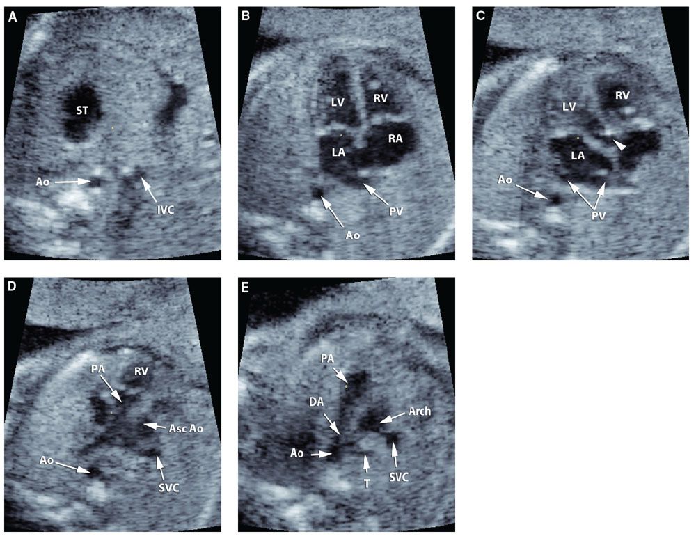
FIGURE 2.27: A: Transverse view of the fetal abdomen; B: Four-chamber view; C: Five-chamber view; D: three-vessel view; E: three-vessel and trachea view. ST, stomach; Ao, descending aorta; IVC, inferior vena cava; RV, right ventricle; LV, left ventricle; RA, right atrium; LA, left atrium; PV, pulmonary veins; PA, pulmonary artery; Asc Ao, ascending aorta; SVC, superior vena cava; T, trachea; DA, ductus arteriosus. Short arrow: aortic root.
Multiple Slice Method: An alternative way to simultaneously display multiple equally spaced planes of section in the same screen is to use the multiple slice method.26
Related posts:
Stay updated, free articles. Join our Telegram channel

Full access? Get Clinical Tree


