Table 1.2

Selected Safety Recommendations for Diagnostic Ultrasound

From Fowlkes JB; Bioeffects Committee of the American Institute of Ultrasound in Medicine. American Institute of Ultrasound in Medicine consensus report on potential bioeffects of diagnostic ultrasound. J Ultrasound Med. 2008;27:503–515. National Council on Radiation Protection and Measurements. Exposure Criteria for Medical Ultrasound, II: Criteria Based on All Known Mechanisms. Bethesda, MD: National Council on Radiation Protection and Measurements; 2002. NRCP report 140.

Effective prenatal diagnosis relies on a high standard of imaging. Several national and international bodies have described standards for imaging in the first, second, and third trimester of pregnancy. These include organizations such as the American College of Obstetricians and Gynecologists (ACOG), American Institute of Ultrasound in Medicine (AIUM), Australasian Society of Ultrasound in Medicine (ASUM), National Health Service (NHS) in the United Kingdom, and the International Society of Ultrasound in Obstetrics and Gynecology (ISUOG) (Table 1.3).^3–7 Guidelines typically describe the essential components of an obstetric ultrasound examination. However, many experts in the field advocate the use of additional views to improve diagnostic performance. In addition to describing the basic components of an obstetrical ultrasound examination in this chapter, we also present extended views that improve the quality of the examination and the detection of pregnancy-related problems. This chapter deals with normal fetal anatomy; however, frequent references to anomalies are made to underscore the pertinence of a good anatomic evaluation. Each image used in this chapter was obtained using two-dimensional (2D) ultrasound. Three-dimensional (3D) ultrasound can be a useful adjunct to 2D ultrasound in select circumstances and will be discussed in Chapter 2. All stated gestational ages are according to last menstrual period dating.

EARLY FIRST TRIMESTER SCAN (5 TO 10 WEEKS’ GESTATION)

The embryonic stage, ending at 10 weeks’ gestation, is a time of very rapid change in the small, developing conceptus.⁴⁵ Ultrasound before 11 weeks’ gestation is not typically regarded as a routine part of pregnancy assessment. When performed, the examination is generally limited to determination of the location and number of gestations present, determination of chorionicity in cases of multiple gestations, assessment for viability, and estimation of gestational age.⁴⁶ Although the anatomy of embryo is not typically examined in detail, a variety of severe congenital anomalies (e.g., severe amniotic band syndrome, body-stalk anomalies, and conjoined twins) may be identified even at this point. A finding that is commonly seen in the early first trimester and that deserves special mention is physiologic herniation of the midgut into the root of the abdominal cord insertion (Fig. 1.1).⁴⁷ This finding is considered normal until the early portion 12th week of gestation and should not be mistaken for an omphalocele.

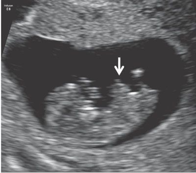
FIGURE 1.1: Sagittal view of a 10- to 11-week fetus demonstrating a physiologic midgut herniation (arrow).

Most examinations at this stage are performed for a specific clinical indication such as pain or vaginal bleeding associated with a positive pregnancy test. Systematic evaluation is needed to accurately distinguish between a viable intrauterine pregnancy, a miscarriage, or an ectopic pregnancy. Ultrasound findings are frequently best interpreted in combination with quantitative maternal serum hCG (human chorionic gonadotropin) with or without progesterone levels. Serial examinations may be needed to reach a diagnosis. The transvaginal approach should be used in all circumstances where a viable intrauterine pregnancy is not obvious on transabdominal assessment. The uterus and adjacent structures should be assessed in both longitudinal and axial sections, taking care to pass completely from side to side and from fundus to cervix to determine the number and location of gestational sacs and embryos. In the early first trimester, the transvaginal approach is ideal to detect any adnexal pathology or free fluid.

Using transvaginal ultrasound, the presence of an intrauterine gestational sac can be consistently demonstrated by the completion of the 5th week of gestation. At this early stage, the gestational age is being estimated by determination of the mean sac diameter (MSD): the average of the sac length, width, and depth. The yolk sac becomes visible within the gestational sac by the midportion of the 6th gestational week, corresponding to an MSD of approximately 10 mm. An embryonic pole with a heartbeat is generally detected by the middle of the 7th gestational week (MSD of approximately 18 mm). When an embryonic pole becomes identifiable, the best method of establishing the gestational age is measurement of the crown-rump length (CRL). Prior to the completion of the 7th gestational week, the anatomy of the embryonic pole is difficult to clearly delineate. At this stage, the CRL is defined as the longest dimension of the embryonic pole (Fig. 1.2). Beginning with the 8th week of gestation, the embryonic head and torso become identifiable. At this point, the CRL is defined as measurement between the top of the fetal head and the fetal rump along its longitudinal axis (Fig. 1.3).⁴⁸ Whereas some investigators advocate using the average of three CRL measurements to establish gestational age, most use the single best measurement. In the 11th week of gestation, the fetus begins to flex and extend its body to a degree that may significantly affect CRL; therefore, CRL measurements need to be carefully standardized from this point on (Fig. 1.4).^49,50

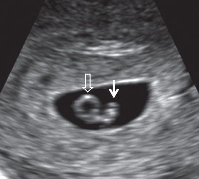
FIGURE 1.2: Embryo at 6.5 weeks’ gestation. Solid arrow, embryo; open arrow, yolk sac.

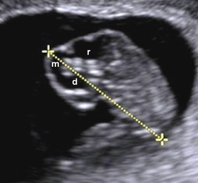
FIGURE 1.3: Sagittal view of an 8-week gestation. Calipers, CRL measurement; d, diencephalon; m, mesencephalon; r, rhombencephalon.

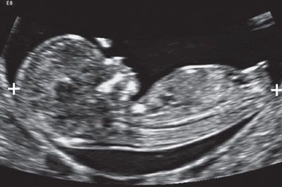
FIGURE 1.4: Sagittal view of an 11- to 12-week fetus. The fetus is in a neutral position and occupies the majority of the image. Calipers, CRL measurement.

The accuracy of CRL measurement decreases with gestational age. Between 7 and 11⁺⁶ weeks’ gestation measurements should be within 4 days of dates by LMP (last menstrual period). At 12 to 13⁺⁶ weeks, an error of ±7 days is considered to be acceptable.^51,52

LATE FIRST TRIMESTER SCAN (11⁺¹ TO 13⁺⁶ WEEKS’ GESTATION)

The late first trimester scan is generally considered to be the first scheduled point for routine ultrasound assessment in pregnancy. It provides the same information as the early first trimester scan with a number of additional benefits. Since it includes highly accurate estimation of gestational age, routine implementation of the late first trimester scan would lead to a significant reduction in postterm pregnancies. During this time frame, the fetus reaches a size and stage of development sufficient to allow for the performance of an informative anatomic survey.^10,11,53 A number of markers, the most important of which is the nuchal translucency measurement, can be employed to provide an accurate risk assessment for aneuploidy. It should also be stressed that an increased translucency and the presence of other markers, most notably tricuspid valve regurgitation and an abnormal ductus venosus (DV) Doppler waveform, increase the risk of structural abnormalities even in chromosomally normal fetuses.⁵⁴

Optimal timing of the first trimester scan involves some compromise. Nuchal translucency assessment is easier to perform and more sensitive at an earlier gestation (11 to 12 weeks), whereas anatomy is best assessed at a slightly later gestation (12 to 13 weeks).⁸ The examination may be performed transabdominally, and if necessary transvaginally, but a combination of the two approaches often yields the best results. Regardless of the approach used, the fetus needs to be assessed in all planes: Longitudinal, axial, and coronal.

The midsagittal section of the fetus is very important, as this allows accurate measurement of CRL and, when adequately magnified, nuchal translucency (Fig. 1.5). Nuchal translucency measurement is typically increased in fetuses affected by chromosomal abnormality. Measurement according to standardized methodology allows individualized levels of risk for trisomy 21, 18, and 13 to be calculated. Another marker for aneuploidy, the fetal nasal bone, can be examined in the same section. Absence of the nasal bone is associated with an increased risk of trisomy 21.⁵⁵ Similarly, the intracranial anatomy of the posterior fossa can be examined and used to screen for spina bifida in this view.¹² The methodology for assessment of these features as well as the overall utility of the 11 to 13⁺⁶ week scan is discussed in detail in Chapter 8.

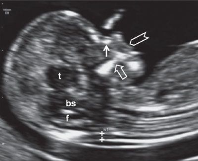
FIGURE 1.5: Sagittal view of a 12- to 13-week fetus. The fetal head and upper torso occupy the majority of the image, and the fetus is in a neutral position. Calipers, NT measurement; solid arrow, nasal bone; t, thalamus; bs, brain stem; f, fourth ventricle; open arrow, maxilla; chevron, upper lip.

Fetal anatomy is most readily assessed with a transverse sweep, running from head to toe. In this section, the intracranial anatomy essentially consists of the lateral ventricles and a very thin layer of brain parenchyma. The lateral ventricles are essentially filled by choroid plexi, which are seen as paired echogenic structures, one within each hemisphere (“butterfly view”). The midline falx is visible as an echogenic line running anteroposteriorly in the midline bisecting the “butterfly” (Fig. 1.6). The posterior fossa contains the developing cerebellum. Since the cerebellar vermis is not yet fused, a large midline communication is seen between the developing fourth ventricle and the cisterna magna (CM) (Fig. 1.7). The posterior fossa undergoes rapid change during the late first trimester, and by 13 to 14 weeks the cerebellum begins to assume a shape resembling that seen in the mid-second trimester (Fig. 1.8). Occasionally, the third ventricle can be detected in a midcoronal section of the head (Fig. 1.9).

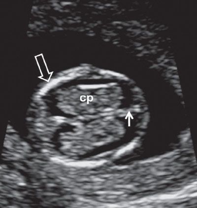
FIGURE 1.6: Axial view of the fetal head at 12 weeks’ gestation. cp, choroid plexus; solid arrow, falx cerebri; open arrow, ossified portion of calvarium.

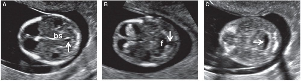
FIGURE 1.7: Transverse views of a fetal head at 12 weeks’ gestation demonstrating hindbrain appearance at various levels in descending order. A: Arrow, developing aqueduct of Sylvius; bs, brain stem. B: Arrow, open communication with cisterna magna; f, fourth ventricle. C: Arrow, cisterna magna.

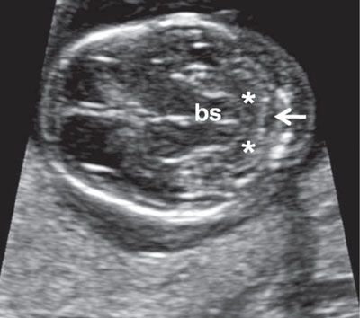
FIGURE 1.8: Transverse views of a fetal head at 13.5 weeks’ gestation demonstrating progressive development of the cerebellum. Compare with Figure 1.7. bs, brainstem; asterisks, cerebellar hemispheres; arrow, cisterna magna.

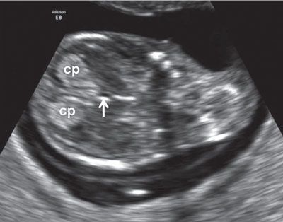
FIGURE 1.9: Midcoronal view of the head at 12 to 13 weeks’ gestation. cp, choroid plexus; arrow, third ventricle.

After 11 weeks’ gestation, the calvarium should be ossified and is seen as an echogenic ring around the intracranial structures (see Fig. 1.6). Absence of an ossified calvarium in association with abnormal intracranial anatomy is consistent with exencephaly/anencephaly sequence. As the transducer is moved caudally, the orbits can be identified. However, these are often better seen in a coronal section of the face (Fig. 1.10). The face, specifically lips and nose, are best examined in sagittal section (see Fig. 1.5). In this view, an upper lip seen extending beyond the tip of the nose raises the possibility of cleft lip and palate.

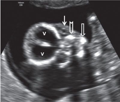
FIGURE 1.10: Coronal view of the fetal face. v, lateral ventricles; solid arrow, ocular orbit with a lens within it; chevron, maxilla; open arrow, body of the mandible.

In an axial section at the superior aspect of the thorax, clavicles can be seen even early in gestation (Fig. 1.11). The four-chamber view and outflow tracts can be assessed using both grayscale and color Doppler imaging (Figs. 1.12 to 1.14). The stomach should be visible in the upper abdomen, and the integrity of the diaphragm can be assessed in sagittal or coronal sections (Figs. 1.15 and 1.16). Returning to an axial section, the anterior abdominal wall and cord insertion are evaluated (Fig. 1.17). The kidneys are generally difficult to see owing to their small size and echogenicity, which is similar to that of the small bowel. Both axial and coronal views are often required in order to identify them with confidence (Figs. 1.18 and 1.19). Color Doppler may be used to look for the renal arteries. However, it should be kept in mind that since the vessels are very small, only small adjustments of the transducer can affect their visualization (Fig. 1.20).^56,57

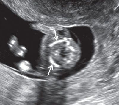
FIGURE 1.11: Transverse view of the lower neck at 12 to 13 weeks’ gestation. Solid arrows, clavicles.

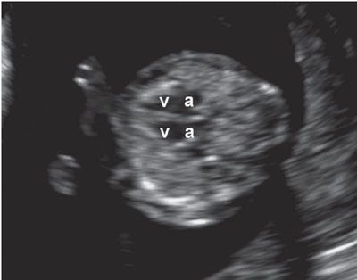
FIGURE 1.12: Transverse view of the chest at 12 to 13 weeks’ gestation containing a four-chamber heart view. v, ventricles; a, atria.

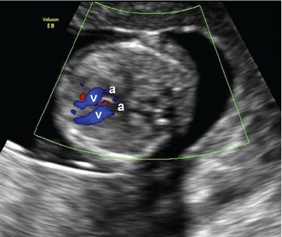
FIGURE 1.13: Transverse view of the chest at 12 to 13 weeks’ gestation containing a four-chamber heart view in diastole with the ventricles (v) highlighted using color Doppler. a, atria.

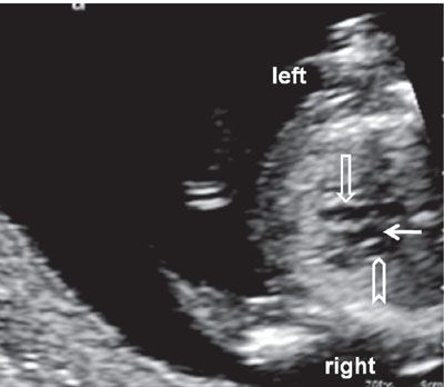
FIGURE 1.14: Transverse view of the chest at 12 to 13 weeks’ gestation at the level of the three-vessel view. Open arrow, pulmonary artery; solid arrow, aorta; chevron, superior vena cava.

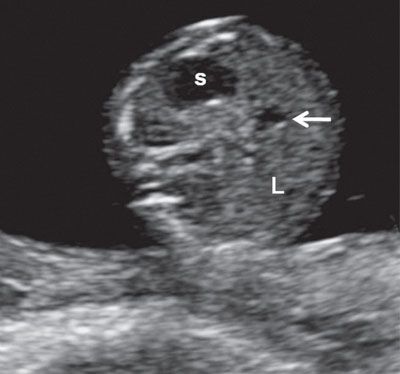
FIGURE 1.15: Transverse view of the abdomen at 13 weeks’ gestation at the level of the abdominal circumference. s, stomach; L, liver; arrow, portal sinus.

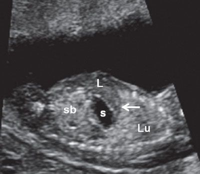
FIGURE 1.16: Left longitudinal view of the abdomen at 12 weeks’ gestation demonstrating the left lung (Lu), intact diaphragm (arrow), left lobe of the liver (L), stomach (s), and small bowel (sb). Note the difference in echogenicities between the various organs.

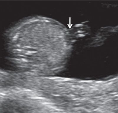
FIGURE 1.17: Transverse view of the abdomen at 13 weeks’ gestation at the level of abdominal cord insertion (arrow).

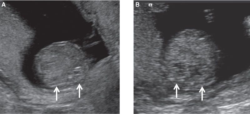
FIGURE 1.18: Transverse view of the abdomen at the level of the kidneys (arrows) at 12 weeks’ gestation (A) and at 13 weeks’ gestation (B).

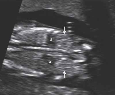
FIGURE 1.19: Coronal view of the abdomen at 12 weeks’ gestation at the level of the kidneys (arrows). Note the relatively prominent adrenal glands (a), which need to be kept in mind in order not to mistake them for the kidneys.

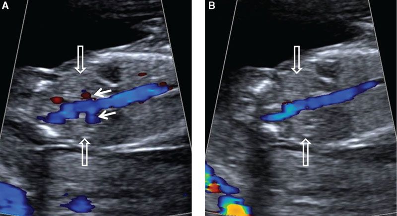
FIGURE 1.20: Coronal view of the abdomen at the level of the kidneys (open arrows) in a 12- to 13-week fetus. Color Doppler is used to demonstrate the renal arteries (solid arrows) in A, which can become nondetectable with only a slight adjustment of the transducer, as in B.

The bladder should be visible in all cases from 12 weeks’ onward. It is best assessed in the midsagittal section. A standardized longitudinal measurement of the bladder in the first trimester should be performed in this view if it appears to be enlarged.⁵⁸ The same section provides information regarding fetal gender by qualitative evaluation or measurement of the angle between the genital tubercle and the fetal longitudinal axis. A small angle, which is essentially parallel to the longitudinal axis of the fetus, indicates a female gender, whereas an angle measuring 30° or more suggests a male gender (Figs. 1.21 and 1.22). Using this method, the accuracy of sex determination is only 70% at 11 weeks’ gestation but increases to nearly 100% at 13 to 14 weeks’ gestation.⁵⁹

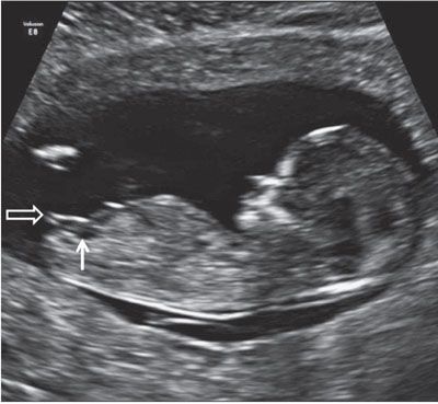
FIGURE 1.21: Sagittal view of a 12- to 13-week fetus demonstrating the presence of a small urinary bladder (solid arrow). The genital tubercle (open arrow) points in a direction parallel to the longitudinal axis of the fetus, indicating a female gender.

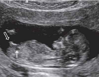
FIGURE 1.22: Sagittal view of a 12- to 13-week fetus demonstrating the presence of a small urinary bladder (solid arrow). The genital tubercle (open arrow) up from the fetal longitudinal axis (>30°).

A skeletal survey is best performed by utilizing both axial and transverse sections. Both hands are commonly held in front of the chest or fetal face, and the legs are generally flexed at the hip at this gestation. The number of fingers is relatively easy to assess in the first trimester as all fingers, including the thumb, lie in approximately the same ultrasound plane (Fig. 1.23). Fetal feet can also be identified, though evaluating the number of toes may be difficult because of their small size (Fig. 1.24). There is a tendency of the ankles to turn inward, making the diagnosis of clubfoot in the first trimester challenging. Both the femur and the humerus can be identified and measured (Figs. 1.25 and 1.26).

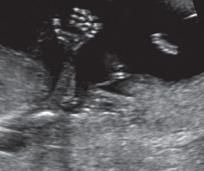
FIGURE 1.23: Fetal hand with all phalangeal ossification centers visible (13 to 14 weeks’ gestation).

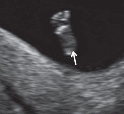
FIGURE 1.24: Fetal foot (arrow) with all five toes visible (12 to 13 weeks’ gestation).

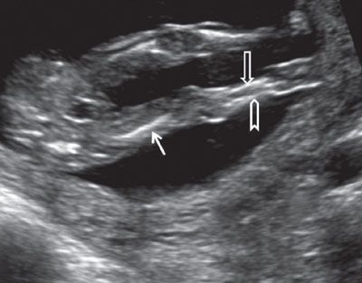
FIGURE 1.25: Both lower extremities visible at 13 to 14 weeks’ gestation. Solid arrow, femur; open arrow, tibia; chevron, fibula.

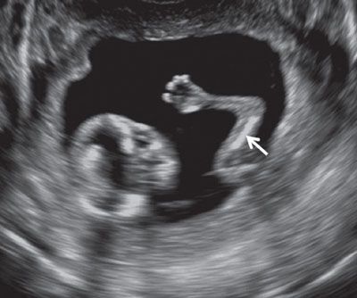
FIGURE 1.26: Upper extremity at 12 to 13 weeks’ gestation. Arrow, humerus.

Color Doppler may be used to help define the cord insertion and the number of arteries in the cord (Fig. 1.27). It can also be used to localize the DV in a right parasagittal section, allowing pulse wave assessment of this vessel for aneuploidy and cardiac screening. The hepatic artery peak systolic velocity may be evaluated in the same section to aid in aneuploidy risk assessment (Fig. 1.28).⁸ Doppler examination involves higher power levels and consequently should generally be avoided during the embryonic period (≤10 weeks’ menstrual gestational age) unless the benefits clearly outweigh the risks. When using Doppler during the 11 to 13⁺⁶ week scan, power indices should be reduced to a minimum, and the region of interest should be interrogated for the minimum time necessary. Often, the region of interest can be effectively identified using grayscale prior to employing Doppler, resulting in reduced energy exposure to the fetus.

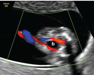
FIGURE 1.27: Transverse/oblique section of the lower abdomen and the pelvis showing the urinary bladder (b) with two umbilical arteries coursing around it in a 12- to 13-week fetus.

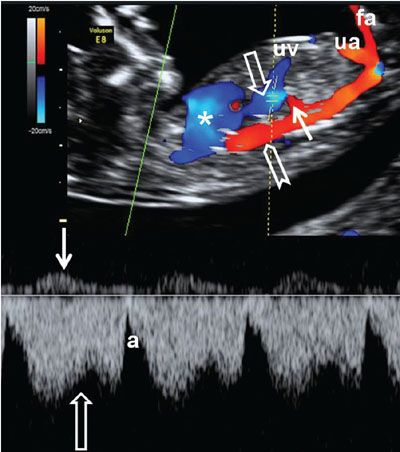
FIGURE 1.28: Right parasagittal section of a fetus at 12 to 13 weeks’ gestation with color and pulsed Doppler. Asterisk, heart; chevron, aorta; open arrows, ductus venosus and its corresponding waveform; solid arrows, hepatic artery and its corresponding waveform; uv, umbilical vein; ua, umbilical artery; fa, femoral artery.

ASSESSING FETAL ANATOMY DURING THE SECOND AND THIRD TRIMESTERS

Standard assessment of the fetus is quite complex. It is best to develop a systematic approach to the examination. A complete examination of the uterine contents in pregnancy includes much more than evaluation of the fetal anatomy; the remaining issues will be discussed in later chapters. The issue of fetal biometry is discussed in this chapter only to illustrate the proper technique rather than clinical applicability.

Fetal anatomy is best assessed at 20 to 24 weeks’ gestation. At this point, the pregnant uterus is out of the pelvis and is located well within the maternal abdomen. The fetus usually presents itself in a better axis for examination. The fetus is also larger and more developed, making the detection of anomalies easier.^60–73 In some jurisdictions, the anomaly scan is performed earlier (e.g., at 18 to 20 weeks’ gestation) in view of the legal restrictions related to interruption of pregnancy if there are abnormal findings. However, it should be pointed out that there is a statistically significant difference in being able to complete the fetal anatomic survey if it is performed at 18 to 18+6 (in 76% of cases) versus 20 to 22+6 weeks’ gestation (in 90% of cases).⁷⁴

The approach to the anatomical survey is essentially the same in both the second and the third trimesters. However, fetal position, reduction in amniotic fluid volume, and increased bony ossification often make the third trimester examination more challenging. It is, however, good practice to briefly check fetal anatomy at the third trimester scan, even if a more comprehensive survey has previously been done at 20 to 24 weeks. Some anomalies may be more readily detectable with the fetus in a different position and others (e.g., duodenal atresia, X-linked aqueductal stenosis, certain skeletal dysplasias, and fetal tumors) generally only become apparent after the mid-second trimester examination. The exact timing of the examination may also depend on maternal habitus. Increased BMI can significantly compromise the ultrasound examination and may require a change in the usual strategy. One reasonable approach to evaluating a fetus in an obese patient is to perform a thorough examination at 12 weeks’ gestation using the transvaginal route and delay the anomaly scan until 22 to 24 weeks’ gestation to increase the likelihood of successfully completing the structural examination.

Immediately after starting the scan, the fetal heart is checked, establishing viability and providing some reassurance to the mother. The uterus should then be scanned in cross section, from left to right and from top to bottom, determining the number of fetuses that are present and defining the lie of the fetus. Placental site and cervical length can then be assessed, although true cervical assessment requires a transvaginal approach, which is best performed at the end of the examination.

Standard fetal biometry includes the following measurements: biparietal diameter (BPD), head circumference (HC), abdominal circumference (AC), and femur length (FL).^75–80 Other measurements that are commonly performed as a part of a routine examination in some centers are the humerus length (HL) and the transcerebellar diameter (TCD).^81,82 The correct manner in which each of these measurements should be obtained is described in the individual sections below. Additional fetal biometry is performed if clinically appropriate. Standard measurements of essentially all fetal structures have been published.

Calvarium

The shape, measurements, and integrity of the calvarium are best assessed utilizing axial and sagittal views. In the axial section, the contour of the fetal head is normally oval in shape. In order to assess the symmetry of the two halves of the brain, regardless of the level of the axial view, care should be taken to keep the falx cerebri truly in the midline. The BPD is assessed using an axial image of the head at a level where standard anatomic landmarks are visible: The globular and slightly hypoechoic paired structures representing the thalami in the midportion of the head with a slit-like hypoechoic structure representing the third ventricle located between them, the cavum septi pellucidi (CSP) in front of the thalami, and the lateral ventricles, with the frontal horns seen anteriorly and the atria (trigones) seen posteriorly. Care should be taken with caliper placement as the authors of some charts measure from the outer aspect of the calvarium in the near field to the inner aspect of the calvarium in the far field, while others use an outer–outer approach. The HC is measured by tracing around the outside of the calvarium in the same axial section as the BPD. In addition to measuring the BPD and HC, the occipitofrontal diameter (OFD) can be measured and expressed in ratio to the BPD (BPD/OFD) as the cephalic index (CI) (Fig. 1.29). This ratio is valuable in describing the shape of the head. The normal range for CI is 0.74 to 0.83. A CI, which is below 0.74, connotes a relatively flat head (dolichocephaly), while a CI above 0.83 describes a relatively round head (brachycephaly).⁸³ Dolichocephaly is not uncommon and is often seen in fetuses that are in a persistently breech presentation or in association with chronic oligohydramnios. Dolichocephaly has been reported in fetuses with sagittal synostosis. Brachycephaly may also be a normal variant but has been described in association with trisomy 21. It can also be seen in conditions where the skull is poorly ossified such as certain types of osteogenesis imperfecta and hypophosphatasia. In these conditions, the skull is also easily compressible, which can be demonstrated by applying gentle pressure with the ultrasound transducer.

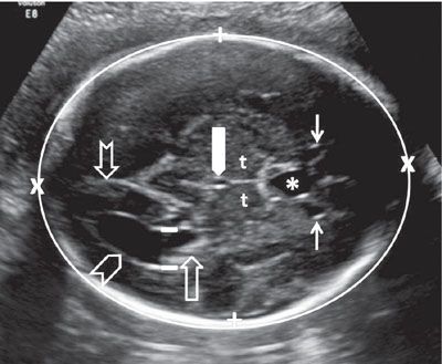
FIGURE 1.29: Axial view of the fetal head at the BPD level. Calipers, BPD measurement; chevron, lateral ventricle (occipital horn); open arrow, lateral ventricle (atrium containing echogenic choroid plexus); thin solid arrows, lateral ventricle (frontal horns); notched arrow, lateral ventricle (occipital horn); thick solid arrow, third ventricle; t, thalamus; asterisk, cavum septi pellucidi. Please note the difference in anatomic detail between the proximal and distal half of the brain.

The shape of the skull may be abnormal in association with a number of specific fetal anomalies. In the mid-second trimester, bifrontal scalloping occurs in >95% of open neural tube defects resulting in a “lemon”-shaped calvarium seen in the axial section.^84,85 The occipital portion of the skull is typically flattened in trisomy 18, while the frontal and parietal portions of the skull gently slope toward one another anteriorly, creating a “strawberry” shape in axial view. Premature closure of multiple cranial sutures restricts expansion of the skull, particularly with advancing gestation, resulting in a “cloverleaf” appearance. The sagittal section offers the best view of the fetal forehead. Abnormalities such as frontal bossing, which are part of a number of skeletal dysplasias or a sloping forehead present in conditions such as microcephaly, are best visualized in this fashion.

The calvarium should be systematically examined to ensure that it is intact. The most common defects are a cephalocele or an encephalocele. These are generally located in the occipital portion of the calvarium, but can be seen less frequently in the area of the nasal root anteriorly or parietally. Disruption of the skull can also occur at more unusual sites, especially when it is caused by amniotic bands. The calvarium will be completely absent in anencephaly.

Intracranial Anatomy

Intracranial anatomy is complex and gestational age–dependent owing to rapid embryologic and later fetal development.⁸⁶ The sections most commonly employed to look at the fetal anatomy are axial ones. This is because of the fact that they are the easiest to obtain and are very familiar to operators who are involved in fetal scanning.

The half of the brain that is closest to the transducer is much more difficult to image clearly when compared with the distal half. This is due to ossification of the skull, which casts an acoustic shadow over the proximal portion of the fetal brain. With advancing gestation, increasing calcification of the calvarium limits resolution. Images can often be improved by rotating the probe so the brain is imaged through the suture lines and fontanelles, using techniques similar to those applied during neonatal examination. Employing the transvaginal route to image a fetus that is cephalic in presentation can facilitate a detailed examination of the intracranial anatomy.

The general symmetry of the fetal brain is first assessed using standard axial views. The presence and position of the falx cerebri should be noted. The falx cerebri is seen as an echogenic line running in the anteroposterior direction. It is a structure that is usually very easy to visualize, and if absent, the possibility of a severe structural defect such as alobar holoprosencephaly should be entertained. The cerebral cortex is a hypoechoic structure, which is fairly thin and difficult to visualize at early gestations. The proportion of the cranial cavity that it fills progressively increases as the gestation advances. The structures that are easiest to identify because of their well-delineated boundaries and greatest differences in echogenicity from the surrounding cortex are the lateral ventricles and the CSP. Routine examination of the intracranial anatomy should always include identification of these structures.

Each lateral ventricle is divided into five parts: The frontal horn, the body of the lateral ventricle, the occipital horn, the inferior (temporal) horn, and the atrium (trigone). The atrium is the point of confluence between the occipital horn, inferior horn, and the body of the lateral ventricle and is the largest, most easily identifiable portion of the lateral ventricle. In axial section at the level of the thalami, the atrium can be measured. This is normally done at the level of the posterior margin of the choroid plexus using a magnified image so that calipers can be accurately placed on the inner margins of the ventricular walls (Fig. 1.29). Enlargement of the lateral ventricle (ventriculomegaly) will be recognized by measurement at this point. At 20 weeks’ gestation, the upper limit of normal is considered to be 10 mm, although recently some authors have suggested that even measurements up to 12 mm are very unlikely to be associated with significant pathology.^87–90 The ventricles become less prominent with advancing gestation although a threshold of measurement <10 mm is typically also used in the third trimester.

It needs to be kept in mind that the shape of the lateral ventricle is 3D complex; unless it is enlarged, it is difficult to visualize in its entirety in a single ultrasound plane. The atrium is located medially. The body and the anterior horn of the lateral ventricle radiate anteriorly, superiorly, and laterally from the atrium. The occipital horns project posteriorly. The temporal horn extends from the atrium in an inferior and anterior direction. Additionally, the bodies of the lateral ventricle and their continuation, the frontal horns, are domed in shape in the sagittal section; therefore, their appearance differs significantly when viewed in various axial planes. The inferior (temporal) horns run through the area of the temporal lobe and are difficult to identify unless they are enlarged. The shape of the ventricles is best assessed using the combination of longitudinal and coronal views (Figs. 1.30 to 1.33). The atrium contains a globular and echogenic structure, the glomus of the choroid plexus. In the majority of cases, the glomus is homogeneous in its ultrasound appearance. However, occasionally echolucent structures of varying complexity and size called choroid plexus cysts (CPCs) are present.^91–93 They can develop in any portion of the choroid plexus, but those that are ≥3 mm tend to be located in the glomus. Unilateral or bilateral CPCs are a common finding affecting 1% to 4% of euploid fetuses but have also been associated with aneuploidy, particularly trisomy 18. They invariably resolve spontaneously and do not represent a true pathologic entity. When found in isolation, risk for aneuploidy is not increased, but it is worth reviewing the results of first trimester screening, and in particular of first trimester biochemistry (both free β-hCG (beta human chorionic gonadotropin) and PAPP-A (pregnancy-associated plasma protein A) are low in trisomy 18), to check there are no common themes through different modalities of screening. The choroid plexus does not extend into the anterior horn of the lateral ventricle; therefore, cystic structures seen anterior to the caudothalamic notch will have a different underlying etiology.

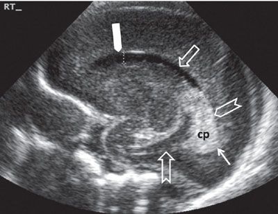
FIGURE 1.30: Sagittal view of the lateral ventricle at 24 weeks’ gestation. Note that this is a neonatal image to show the anatomy in its entirety. cp, choroid plexus; thick solid arrow, frontal horn; open arrow, body of the lateral ventricle; chevron, trigone; thin solid arrow, portion of the occipital horn; notched arrow, inferior (temporal) horn.

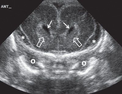
FIGURE 1.31: Anterior coronal view of the brain at 24 weeks’ gestation. Please note the increased amount of extra-axial fluid, which is normal early in gestation. Note that this is a neonatal image to show the anatomy in its entirety. Solid arrows, frontal horns of the lateral ventricles; open arrows, caudate nuclei; o, orbit; asterisk, extra-axial fluid.

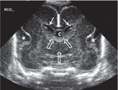
FIGURE 1.32: Midcoronal view of the brain at 24 weeks’ gestation. Please note the increased echogenicity of the roof of the third ventricle extending into the foramina of Monro. This represents the choroid plexus. Note that this is a neonatal image to show the anatomy in its entirety. Thin solid arrows, bodies of the lateral ventricles; thick solid arrow, corpus callosum; open arrows, location of the foramina of Monro; notched arrow, third ventricle; asterisk, operculization of the insula; c, cavum septi pellucidi.

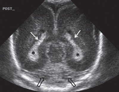
FIGURE 1.33: Posterior coronal view of the brain at 24 weeks’ gestation. Note that this is a neonatal image to show the anatomy in its entirety. White arrows, trigones; asterisks, choroid plexi; black arrows, section through a portion of the cerebellum.

The CSP and its posterior extension, the cavum septi vergae (CSV), are seen as a continuous hypoechoic structure located in the midline. It represents a space between the two septi pellucidi, which is filled with cerebrospinal fluid (CSF). Not infrequently, the cavum septi pellucidi et vergae (CSPV) contains septations, especially in its posterior portion (Fig. 1.34). The CSPV begins to close in the third trimester, a process that is completed in infancy.

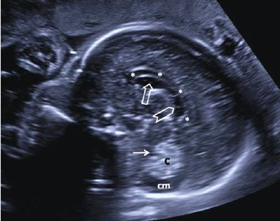
FIGURE 1.34: Sagittal view of the fetal head at 24 weeks’ gestation. Please note the septations in the cavum septi vergae seen as echogenic lines running anteroposteriorly. Asterisks, corpus callosum; open arrow, cavum septi pellucidi; chevron, cavum septi vergae; solid arrow, fourth ventricle; c, cerebellum; cm, cisterna magna.

There is no direct communication between the ventricular system and CSPV; it is diffusion across the thin septi pellucidi that allows CSF to enter this space. This space begins to close in late gestation, a process that is completed during infancy. It is bounded by the corpus callosum anteriorly and superiorly, the fornix posteriorly, and the anterior commissure inferiorly. In a midsagittal section, the CSPV is arched in shape. Therefore, in the standard axial section at the level of the BPD, usually it is only the CSP that is visible. In this section, the CSP appears as a hypoechoic roughly rectangular structure located anteriorly to the thalami. As a normal variant, the CSV can be unusually large and visible in this section. Since the CSPV is arched in shape, may appear to be separate from the cavum septi pellucid, simulating a cyst (Fig. 1.35). Examination of the CSPV in the sagittal section will help to elucidate the diagnosis (see Fig. 1.34). A cystic midline structure that is occasionally seen located posteriorly and inferiorly to the CSV is the cavum veli interpositi (Fig. 1.36). This is a normal variant and is part of the leptomeningeal space between the roof of the third ventricle and the body of the fornices. The size of this structure normally does not exceed 1 cm. It can be difficult to distinguish from an arachnoid cyst located at the quadrigeminal cistern.^94,95

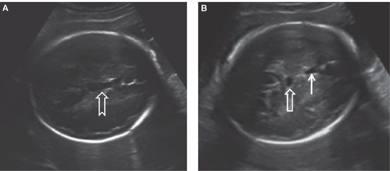
FIGURE 1.35: Axial view of a fetal head at 32 weeks. A: Section through the cavum septum pellucidi et vergae at a point when continuity between two is evident (arrow). B: Axial view in a plane slightly caudal to A, where the cavum septi pellucidi (solid arrow) and cavum septi vergae (open arrow) are seen as two separate structures. The latter should not be mistaken for a cyst.

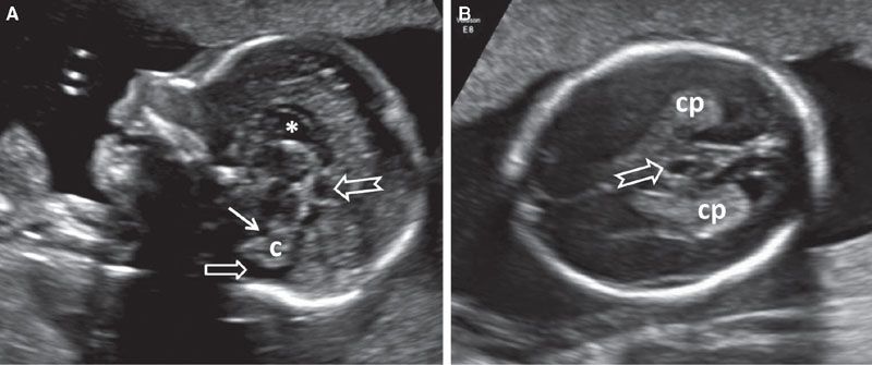
FIGURE 1.36: A: Sagittal section of a fetal head at 22 weeks’ gestation with a cavum veli interpositi (notched arrow) located posteriorly and inferiorly to CSPV (asterisk). Solid arrow, fourth ventricle; open arrow, cisterna magna; c, cerebellum. B: Axial view of the same fetus. Arrow, cavum veli interpositi; cp, choroid plexus.

The importance of positively identifying the CSPV lies in the fact that it can be absent in association with midline defects. It should be remembered that the anterior pillars of the fornices lie in the same general area as the CSP. They are hypoechoic and have a generally rectangular shape in the axial plane. This can lead to a false impression that the CSP is present, consequently missing the diagnosis of anomalies that can be associated with absent CSPV such as agenesis of corpus callosum, septo-optic dysplasia, lobar holoprosencephaly, and neuronal migration defects. However, unlike the CSP, a thin echogenic line can be seen between the two fornices, which helps to differentiate between the two entities (Fig. 1.37).⁹⁶ In the sagittal view, visualization of the pericallosal artery helps to confirm the presence of the corpus callosum (Fig. 1.38). Since the corpus callosum is a structure that completes its formation relatively late in pregnancy, the CSPV should not be expected to be visible prior to 18 to 19 weeks’ gestation.

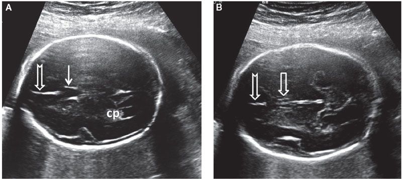
FIGURE 1.37: A: Axial section of a fetal head at 22 weeks’ gestation at the level of the cavum septi pellucidi (solid arrow). Notched arrow, falx cerebri; cp, choroid plexus. B: Axial view of the same fetus in slightly more caudal section. Note the two juxtaposed pillars of the fornix (open arrow) with a midline echogenic division. Notched arrow, falx cerebri.

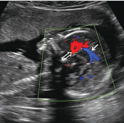
FIGURE 1.38: Sagittal view of the fetal head at 22 weeks. Anterior cerebral (open arrow) and pericallosal (solid arrow) arteries with some of their branches are demonstrated using color Doppler.

The third ventricle is located inferiorly to the CSP, between the paired thalami. This slit-like structure is filled with CSF and is hypoechoic in its ultrasound appearance (see Fig. 1.29). It is normally small (<3 mm diameter) and may be difficult to visualize. Enlargement of the third ventricle is typically only seen in association with enlargement of the lateral ventricles.

Examination of the cerebral cortex focuses on ruling out any space occupying lesions, either cystic or solid in nature. Cortical maturation continues throughout pregnancy, as the brain develops gyri and loses its smooth appearance (Fig. 1.39). The process of cortical maturation can be most easily observed in the insula. Even though operculization of the insula begins at approximately 14 weeks’ gestation, on ultrasound, this process does not become evident until approximately 19 weeks’ gestation. It begins as infolding of the cerebral cortex at the lateral edge of the cerebrum located initially in the anterior half of the distance between the occiput and the forehead. It first appears as a heterogeneous depression, which is increased in echogenicity. Prominent pulsations can be seen at the bottom of the depression, which represents the Sylvian segment of the middle cerebral artery (Fig. 1.40). As operculization progresses, the depression is roofed over by the temporal lobe. By the completion of the process at the beginning of the third trimester, it remains as only a slit-like structure, representing the Sylvian fissure (Fig. 1.41). Absence of normal operculization raises the possibility of a neuronal migration defect such as lissencephaly.

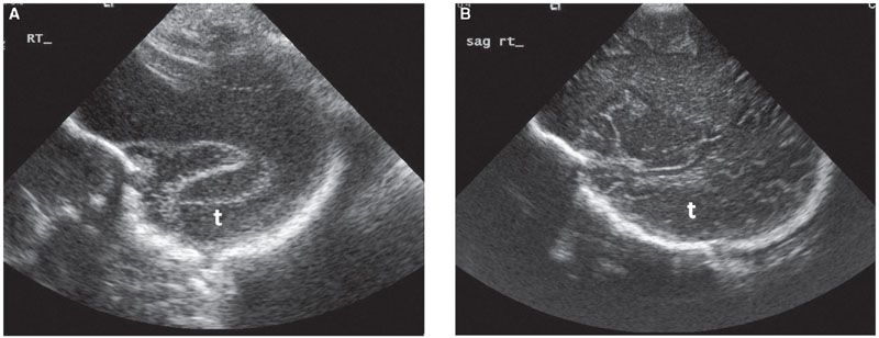
FIGURE 1.39: Parasagittal section of the fetal head with the temporal lobe (t) visible. Please note the difference in the texture of the surface of the cortex, with absent sulci and gyri at 22 weeks’ gestation (A) and well-developed pattern of sulci and gyri at term (B).

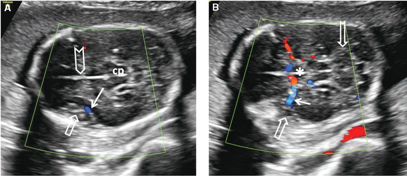
FIGURE 1.40: A: Axial section of a fetal head at 20 weeks’ gestation demonstrating the insula at an early stage of operculization (open arrow) with the middle cerebral artery (color Doppler) at its base (solid arrow). Chevron, falx cerebri; cp, cerebral peduncles. B: Slightly more caudal section of the same fetus demonstrating the course of the middle cerebral artery (solid arrow) to the base of the insula (open arrow) with color Doppler. Asterisk, center of the circle of Willis; notched arrow, cerebellum.

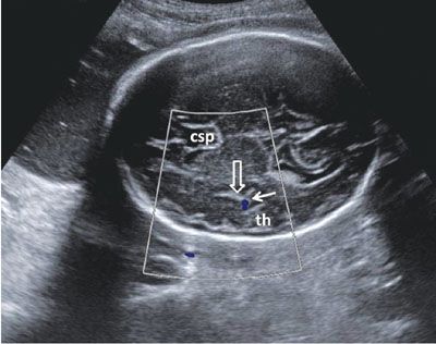
FIGURE 1.41: Axial view of a fetal head in the third trimester after the completion of insular operculization. th, temporal horn; solid arrow, color Doppler of the middle cerebral artery; open arrow, Sylvian fissure; csp, cavum septi pellucidi.

Posterior Fossa

Another axial section routinely employed to evaluate the intracranial anatomy is the suboccipitobregmatic view: Starting with the BPD view, the posterior aspect of the probe is rotated caudally until the posterior fossa becomes visible. Even though this view is primarily designed to evaluate the posterior fossa and the back of the fetal head, it also offers a good view of the CSP, thalami, and the midbrain as well as their anatomic relationship (Fig. 1.42). Sagittal views of the posterior fossa are also very informative. Coronal sections add very little information to the axial ones, but depending on the position of the fetus, this approach may provide the clearest view.

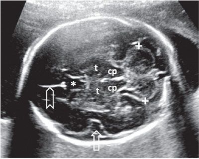
FIGURE 1.42: Suboccipitobregmatic view of the head. Calipers, transcerebellar diameter; cp, cerebral peduncles; t, thalami; open arrow, insula; asterisk, cavum septi pellucidi; chevron, falx cerebri.

Routine examination of the posterior fossa is critical to detect not only anomalies that originate in the posterior fossa but also changes that are indicative of problems in the spine. In addition to the bifrontal scalloping of the cranium described earlier, open spine defects are accompanied by the Chiari Type II malformation (herniation of the cerebellar tonsils through the foramen magnum and downward displacement of the cerebellar vermis). In the axial view, this defect translates into flattening of the cerebellar hemispheres with an anterior bend (so-called banana sign) and obliteration of the CM.^{84,85,97–99} Finally, since most cephaloceles and encephaloceles are located in the occipital region of the skull, examination of the posterior fossa must also include a careful evaluation of the calvarium in that region.¹⁰⁰

The formation of the cerebellar hemispheres and the connecting vermis continues throughout the first half of the pregnancy. Since the vermis is not fully developed until mid-gestation, vermian defects, especially small ones, are difficult to diagnose prior to 18 to 20 weeks’ gestation. Using axial planes, the mid-second trimester cerebellum is seen as a dumbbell-shaped structure consisting of two hemispheres connected by the vermis. The shape of the cerebellar hemispheres becomes somewhat flattened on its anterior surface. As gestation advances, the vermis increases in echogenicity in relation to the hemispheres, and the caudal part of the vermis becomes notched (cerebellar tonsils). The hemispheres develop gyri through the third trimester, which are visible on ultrasound, and the cerebellar tonsils become more elongated. An axial view of the inferior aspect of the cerebellum at this point in pregnancy may reveal a fluid-filled space between the tonsils, which may lead to the erroneous diagnosis of a defect in the vermis. The TCD is measured in an axial section using the suboccipitobregmatic view. Care must be taken so that the cerebellar hemispheres are symmetrical, and the measurement is done at a point where the distance between the lateral edges of the two hemispheres is the greatest.^101,102

Every attempt should be made to visualize both cerebellar hemispheres to allow a comparison of their size and echotexture. There are conditions that may affect only one of the cerebellar hemispheres such as unilateral hypoplasia, hemorrhage, or infarction. If a cerebellar defect or ventriculomegaly is suspected, the fourth ventricle should be evaluated. It is seen as a hypoechoic structure between the cerebral peduncles and the cerebellum (Fig. 1.43). Isolated enlargement of the fourth ventricle is unlikely to occur and is of limited clinical significance.

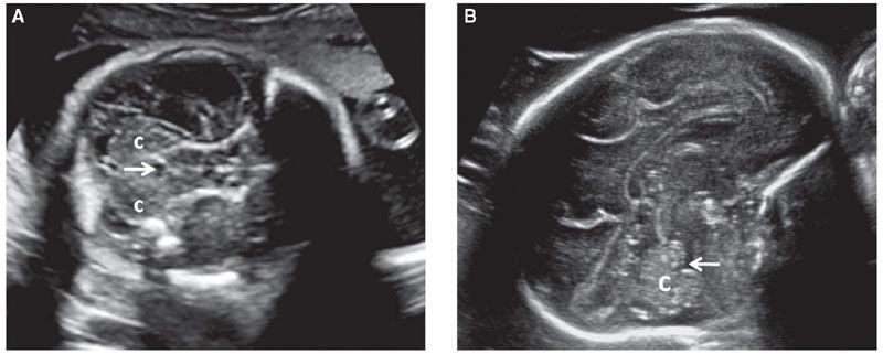
FIGURE 1.43: A: Axial section of a fetal head in the mid-second trimester weeks demonstrating the fourth ventricle (arrow). c, cerebellar hemispheres. B: Sagittal section of a fetal head in the early third trimester. Arrow, fourth ventricle; c, cerebellum.

The CM is a CSF-filled structure that is located behind the cerebellum. If it appears to be exceptionally large, it can be objectively assessed by measurement of its anteroposterior diameter in an axial section of the posterior fossa (Fig. 1.44). Even though normal CM diameter is below 10 mm, isolated CM enlargement (mega-cisterna magna) is considered to be a normal variant. Nonetheless, a large CM should lead to a detailed evaluation of the fetal anatomy overall and the cerebellar vermis specifically, as this finding has a weak association with trisomy 13 and 21 and verminan defects. Septations within the CM are a common finding and occasionally they can simulate a small cyst. These are due to subarachnoid trabeculae and represent a normal finding.^103–105

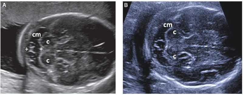
FIGURE 1.44: A, B: Suboccipitobregmatic views of the head demonstrating a variety of normal septations within the cisterna magna (cm). Note the formation of a cyst-like structure in B. Calipers, cisterna magna measurement; c, cerebellar hemispheres.

With the exception of the above-described Chiari Type II malformation, most defects affecting the posterior fossa are cystic in nature (Dandy–Walker malformation, Blake’s pouch, arachnoid cysts, and dysgenesis of the cerebellar vermis). These diagnoses can be difficult to tease out and depend on findings in axial, midsagittal, and coronal sections. The posterior fossa anomalies are one area where a fetal MRI may be especially helpful in arriving at the correct diagnosis.

Finally, the suboccipitobregmatic view is also used as a standardized view for nuchal fold measurement. Thickened (>6 mm) nuchal fold is associated with an increased risk of trisomy 21.

Fetal Spine

Assessment of the central nervous system is not complete without detailed examination of the fetal spine. This involves evaluation of the vertebrae and the contents of the spinal canal. Open spinal defects also disrupt the skin, so careful examination of the cutaneous covering of the spine is also important. The vertebral column should be evaluated in at least two of the three planes: coronal, axial, and longitudinal (midsagittal). The vertebrae have three ossification centers visible prenatally: Vertebral body anteriorly and one in each of the vertebral arches (laminae) posteriorly. In the axial section, the three ossification centers are in a triangular arrangement. The vertebral body ossification center is round and is located in the midline. The paired laminar ossification centers are slightly offset from the midline. They are linear in shape and form a roof over the spinal canal (Fig. 1.45).^106,107 In the presence of an open spine defect, this arrangement is disrupted, and the laminar ossification centers are displaced laterally, forming the shape of the letter U or V in the axial view of the spine. Often, axial views are best for assessing the integrity of the skin. Both individual vertebrae and their skin covering should be evaluated by sliding the transducer along the entire length of the spine.

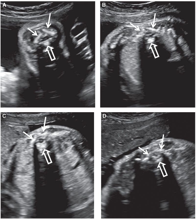
FIGURE 1.45: A transverse view of vertebrae at various levels of the vertebral column: cervical (A); thoracic (B); lumbar (C); sacral (D). The three ossification centers (solid arrows, vertebral arches; open arrow, vertebral body) are seen. Note the differences in their appearance depending on the level.

The whole length of the vertebral column can be seen in both a coronal and in a sagittal section, and the ossification centers should be spaced evenly in these views. In the coronal view, the two lateral points of ossification can be visualized cleanly, and by moving the probe anteriorly, ossification of the vertebral body can be brought into view. As the spine is curved, it is common to be able to visualize the vertebral bodies at some levels and the arches at other levels in the same view (Fig. 1.46). In longitudinal section, the line of ossification of vertebral bodies is seen anteriorly and, if there is a slight oblique cut, one set of posterior ossification sites will be visualized. In the anteroposterior axis, the spine is curved, being convex in the thoracic region and concave in the lumbosacral region. The sacral portion of the spine usually has a more persistent curvature, with the tip of the spine pointing posteriorly (Fig. 1.47). This sacral upswing may be absent in the presence of an open spine defect and in the presence of caudal regression syndrome.

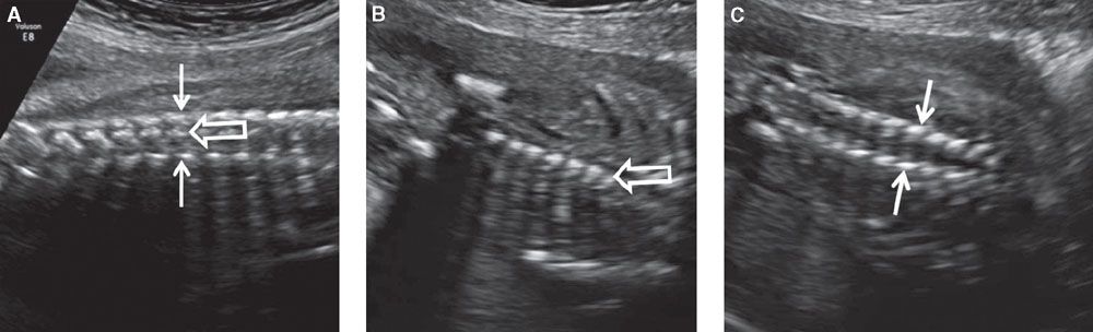
FIGURE 1.46: Coronal views of the vertebral column. A: Section demonstrating all three types of ossification centers in the same view. Solid arrows, vertebral arch ossifications; open arrow, vertebral body ossification. B: Section demonstrating vertebral body ossification centers (open arrow) only. C: Section demonstrating vertebral arch ossification centers (solid arrows) only.

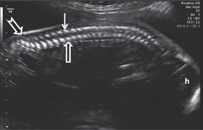
FIGURE 1.47: Sagittal view of the spine in mid-second trimester demonstrating its normal curvature. Open arrow, vertebral body ossification center; solid arrow, vertebral arch ossification center. Note the sacral upswing (notched arrow). h, head.

Overcurvature of the thoracic spine, kyphosis, or lateral curvature of the spine, scoliosis, can be detected by careful assessment of at least two of the three standard planes. Abnormal curvature may be due to the presence of a hemivertebra, which is a feature of a number of genetic syndromes such as VACTERL; therefore, other anomalies known to be associated with this syndrome should be actively sought.

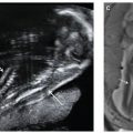
The spinal cord can be delineated within the spinal canal using ultrasound on most exams (Fig. 1.48). However, the presence of multiple vertebral ossification centers does obscure it to a variable degree, especially later in gestation. The ultrasound appearance of the spinal cord is fairly uniform with slightly decreasing size moving cranial to caudal. The conus medullaris can be identified as the place where the spinal cord comes to its end point (Fig. 1.49). Measuring the distance between the tip of the conus medullaris to the tip of the spine is potentially useful in diagnosing tethered cord, and therefore spina bifida occulta.¹⁰⁸ Fetal hair can occasionally be seen on ultrasound, especially in the third trimester.¹⁰⁹ It can also form a prominent echogenic line behind the fetal back generally following the outline of the spine, which may be a confusing finding for those that are not aware of this possibility (Fig. 1.50).

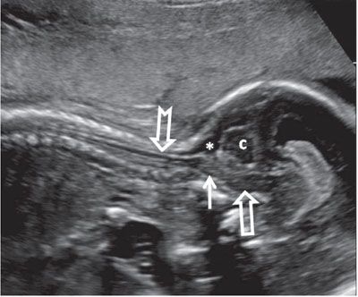
FIGURE 1.48: Sagittal view of the cervical spinal cord (notched arrow) in late second trimester. Solid arrow, medulla oblongata; open arrow, pons; asterisk, cisterna magna; c, cerebellum.

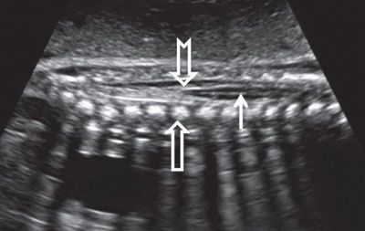
FIGURE 1.49: Sagittal view of the lumbar spinal cord (solid arrow) ending in the conus medullaris (notched arrow) in late second trimester. Open arrow, vertebral body ossification center.

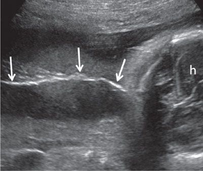
FIGURE 1.50: Superficial coronal view along the fetal back in the third trimester. A thin line of hair along the fetal back (arrows) is seen. h, fetal head.

Fetal Face

The face is a large and complex structure. As such, it needs to be examined at multiple levels and in multiple planes.¹¹⁰

Related posts:

Hydrops First Trimester Evaluation Growth, Doppler, and Fetal Assessment Neck Advanced Assessment of Fetal Cardiac Function Multiple Gestation

Stay updated, free articles. Join our Telegram channel

Join