chapter 15 Image Quality in Nuclear Medicine
Image quality refers to the faithfulness with which an image represents the imaged object. The quality of nuclear medicine images is limited by several factors. Some of these factors, relating to performance limitations of the gamma camera, already have been discussed in Chapter 14. In this chapter, we discuss the essential elements of image quality in nuclear medicine and how it is measured and characterized. Because of its predominant role in nuclear medicine, the discussion focuses on planar imaging with the gamma camera; however, the general concepts are applicable as well to the tomographic imaging techniques that are discussed in Chapters 17 to 19.
A Basic Methods for Characterizing and Evaluating Image Quality
There are two basic methods for characterizing or evaluating image quality. The first is by means of physical characteristics that can be quantitatively measured or calculated for the image or imaging system. Three such characteristics that are used for nuclear medicine image quality are (1) spatial resolution (detail or sharpness), (2) contrast (difference in image density or intensity between areas of the imaged object containing different concentrations of radioactivity), and (3) noise (statistical noise caused by random fluctuations in radioactive decay, or structured noise, e.g., resulting from instrument artifacts). Although they describe three different aspects of image quality, these three factors cannot be treated as completely independent parameters because improvements in one of them frequently are obtained at the expense or deterioration of one or more of the others. For example, improved collimator resolution usually involves a tradeoff of decreased collimator efficiency (see Chapter 14, Section C) and, hence, decreased counting rates and increased image statistical noise.
A related approach, known as computer observer performance studies, uses a mathematical model that under appropriate conditions predicts the performance of a human observer and can be used as a surrogate for actual human observer studies. Because human observer studies require large numbers of images and therefore are very time consuming, computer observers often are more practical. Details regarding computer observer models are beyond the scope of this text and the interested reader is referred to reference 1 for further information.
B Spatial Resolution
1 Factors Affecting Spatial Resolution
Spatial resolution refers to the sharpness or detail of the image, or to the ability of the imaging instrument to provide such sharpness or detail. The sample images presented in Chapters 13 and 14 already have demonstrated that nuclear medicine images have somewhat limited spatial resolution, at least in comparison with photographic or radiographic images. A number of factors contribute to the lack of sharpness in these images.
Collimator resolution is perhaps the principal limiting factor when absorptive collimators are used for spatial localization (Chapter 14, Section C). Because collimator hole diameters must be relatively large (to obtain reasonable collimator efficiency), there is blurring of the image by an amount at least as great as the hole diameters (Equation 14-6). Collimator resolution also depends on source-to-detector distance (Figs. 14-16 through 14-22). Note that collimator resolution is not a factor in positron emission tomography (PET) imaging, which uses annihilation coincidence detection for spatial localization (Chapter 18, Section A).
A second factor is intrinsic resolution of the imaging detector. With the gamma camera, this limitation arises primarily because of statistical variations in the distribution of light photons among the photomultiplier tubes (Chapter 14, Section A.1). Intrinsic resolution is a function of γ-ray energy with the gamma camera, becoming poorer with decreasing γ-ray energy (Fig. 14-2). For imaging devices with discrete detector elements, such as many PET systems (see Chapter 18, Section A.3), the size of the individual detector elements largely determines the intrinsic resolution of the device.
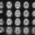
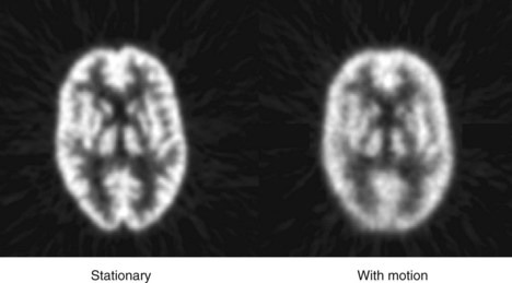
Image sharpness also can be affected by patient motion. Figure 15-1 shows images of a brain phantom obtained with and without motion. Respiratory and cardiac motion can be especially troublesome because of the lengthy imaging times required in nuclear medicine and the relatively great excursions in distance (2-3 cm) that are possible in these instances. Gated-imaging techniques (see Chapter 20, Section A.4) have been employed to minimize motion blurring, especially in cardiac studies. Breath-holding also has been used to minimize blurring caused by respiratory motion.
Nuclear medicine imaging systems acquire data on a discrete matrix of locations, or pixels, which leads to pixelation effects in the image. As discussed in Chapter 20, the size of the discrete pixels sets a limit on the spatial resolution of the image. In general, it is desirable to have at least two pixels per full width at half maximum (FWHM) of system resolution to avoid creating distracting pixelation effects and possible loss of image detail.
2 Methods for Evaluating Spatial Resolution
Spatial resolution may be evaluated by subjective or objective means. A subjective evaluation can be obtained by visual inspection of images of organ phantoms that are meant to simulate clinical images (e.g., the brain phantom in Fig. 15-1). Although they attempt to project “what the physician wants to see,” organ phantoms are not useful for quantitative comparisons of resolution between different imaging systems or techniques. Also, because of the subjective nature of the evaluation, different observers might give different interpretations of comparative image quality.
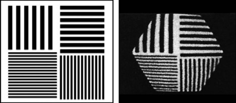
A phantom that can be used for more objective testing of spatial resolution is shown in Figure 15-2. Bar phantoms are constructed of lead or tungsten strips, generally encased in a plastic holder. Strips having widths equal to the spaces between them are used. For example, a “5-mm bar pattern” consists of 5-mm-wide strips separated edge to edge by 5-mm spaces. The four-quadrant bar phantom shown in Figure 15-2 has four different strip widths and spacings. To evaluate the intrinsic resolution of a gamma camera, the bar phantom is placed directly on the uncollimated detector and irradiated with a uniform radiation field, typically a point source of radioactivity at several meters distance from the detector. To evaluate the resolution with a collimator, the phantom is placed directly on the collimated detector and irradiated with a point source at several meters distance, or with a sheet source of radioactivity placed directly behind the bar phantom. Spatial resolution is expressed in terms of the smallest bar pattern visible on the image. There is a certain amount of subjectivity to the evaluation, but not so much as with organ phantoms.
To properly evaluate spatial resolution with bar phantoms, one must ensure that the thickness of lead strips is sufficient so that they are virtually opaque to the γ rays being imaged. Otherwise, poor visualization may be due to poor contrast of the test image rather than poor spatial resolution of the imaging device. For 99mTc (140 keV ) and similar low-energy γ-ray emitters, tenth-value thicknesses in lead are approximately 1 mm or less, whereas for 131I (364 keV ), annihilation photons (511 keV), and so on, they are on the order of 1 cm (see Table 6-4). Most commercially available bar phantoms are designed for 99mTc and are not suitable for use with higher-energy γ-ray emitters.
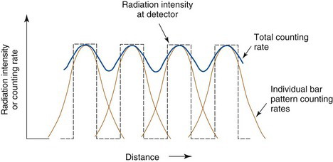
A still more quantitative approach to evaluating spatial resolution is by means of the point-spread function (PSF) or line-spread function (LSF). General methods for recording these functions were described in Chapter 14, Section E.2. Examples of LSFs are shown in Figure 17-8 for a single-photon emission computed tomography (SPECT) camera and in Figure 18-5 for a PET system. Although the complete profile is needed to fully characterize spatial resolution, a partial specification is provided by its FWHM (Fig. 14-15). The FWHM is not a complete specification because PSFs or LSFs of different shapes can have the same FWHM. (Compare, for example, the different shapes in Figs. 18-5 and 18-7). However, the FWHM is useful for general comparisons of imaging devices and techniques. Roughly speaking, the FWHM of the PSF or LSF of an imaging instrument is approximately 1.4-2 times the width of the smallest resolvable bar pattern (Fig. 15-3). Thus an instrument having an FWHM of 1 cm should be able to resolve 5- to 7-mm bar patterns.
In most cases, multiple factors contribute to spatial resolution and image blurring. The method for combining FWHMs for intrinsic and collimator resolutions to obtain the overall system FWHM is discussed in Chapter 14, Section C.4 and in Appendix G. In general, if a system has n factors or components that each contribute independently to blurring, individually characterized by FWHM1, FWHM2, . . ., FWHMn, the FWHM for the system is given by
This equation provides an exact result when all of the components have gaussian-shaped blurring functions, but it is an approximation when nongaussian shapes are involved. Note that if the FWHM for any one factor is significantly larger than the others, it becomes the dominating factor for system FWHM. Thus, for example, if FWHM1  FWHM2, it makes little sense to expend substantial effort toward improving FWHM2.
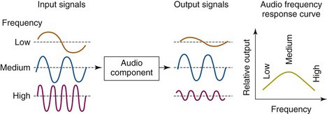
The most detailed specification of spatial resolution is provided by the modulation transfer function (MTF). The MTF is the imaging analog of the frequency response curve used for evaluating audio equipment. In audio equipment evaluations, pure tones of various frequencies are fed to the input of the amplifier or other component to be tested, and the relative amplitude of the output signal is recorded. A graph of relative output amplitude versus frequency is the frequency response curve for that component (Fig. 15-4). A system with a “flat” curve from lowest to highest frequencies provides the most faithful sound reproduction.
By analogy, one could evaluate the fidelity of an imaging system by replacing the audio tone with a “sine-wave” distribution of activity (Fig. 15-5). Instead of varying in time (cycles per second), the activity distribution varies with distance (cycles per centimeter or cycles per millimeter). This is called the spatial frequency of the test pattern, customarily symbolized by k.* The modulation of the test pattern, which is a measure of its contrast, is defined by
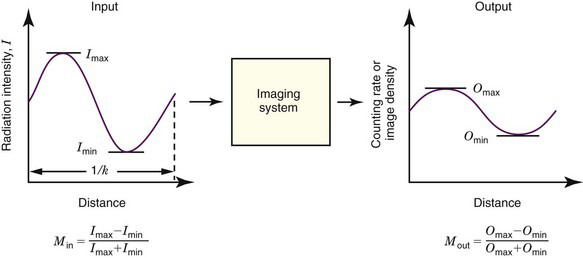


The ratio of output to input modulation is the MTF for the spatial frequency k of the test pattern,
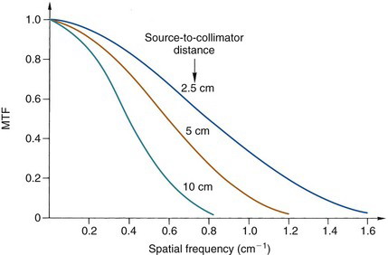
Figure 15-6 illustrates some typical MTF curves for a gamma camera collimator. The MTF curves have values near unity for low frequencies but decrease rapidly to zero at higher frequencies. Thus the images of a radionuclide distribution obtained with this collimator show the coarser details of the distribution faithfully but not the fine details. Edge sharpness, which is a function of the high-frequency MTF values, also is degraded. This type of performance is characteristic of virtually all nuclear medicine imaging systems. Note also that the MTF curve at higher frequencies decreases more rapidly with increasing source-to-collimator distance.
The MTF curve characterizes completely and in a quantitative way the spatial resolution of an imaging system for both coarse and fine details. Images of bar patterns and similar test objects are quantitative only for specifying the limiting resolution of the imaging system, for example, the minimum resolvable bar pattern spacing. Bar-pattern images and MTF curves can be related semiquantitatively by noting that the spatial frequency of a bar pattern having bar widths and spaces of x cm is one cycle per 2x cm. Thus a “5-mm bar pattern” has a basic spatial frequency of one cycle per centimeter (one bar and one space per centimeter). Roughly speaking, bar patterns are no longer visible when the MTF for their basic spatial frequency drops below a value of approximately 0.1. MTF curves thus can be used to estimate the minimum resolvable bar pattern for an imaging system.
In practice, MTFs are not determined using sinusoidal activity distributions, as illustrated in Figure 15-5, which would be difficult to construct. Instead, they are obtained by mathematical analysis of the LSF or PSF. Specifically, the MTF of an imaging system can be derived from the Fourier transform (FT) of the LSF or PSF.* The one-dimensional (1-D) FT of the LSF is the MTF of the system measured in the direction of the profile, that is, perpendicular to the line source. Similarly, the 1-D FT of a profile recorded through the center of the PSF gives the MTF of the system in the direction of the profile. Alternatively, a 2-D FT of the 2-D PSF provides a 2-D MTF that can be used to determine the frequency response of the system at any angle relative to the imaging detector. This sometimes is useful for imaging systems that have asymmetrical spatial resolution characteristics, such as detector arrays with rectangular elements. Some PET detector arrays have this property (see Chapter 18, Section B).
It also is possible to obtain a 3-D representation of the MTF from a complete 3-D data set for the PSF. This is potentially useful for characterizing the spatial resolution of tomographic instruments in all three spatial directions. Note that in all cases the diameter or width of the source should be much smaller than resolution capability of the imaging device (d  FWHM/4). Additional discussions about the measurement of MTFs and their properties can be found in references 2 and 3.

In general, the MTF of a system is the product of the MTFs of its components.
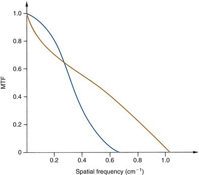
If two systems have MTF curves of the same general shape, one can predict confidently that the system with the higher MTF values will have superior spatial resolution; however, the situation is more complicated when comparing two systems having MTF curves of different shapes. For example, Figure 15-7 shows MTF curves for two collimators, one of which would be better for visualizing large low-contrast structures (low frequencies), the other for fine details (high frequencies). To gain an impression of comparative image quality in this situation, one would probably have to evaluate organ phantoms or actual patient images obtained with these collimators.