1 Annihilation Coincidence Detection

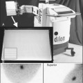
When a positron undergoes mutual annihilation with a negative electron, their rest masses are converted into a pair of annihilation photons (see Fig. 3-7). The photons have identical energies (511 keV) and are emitted simultaneously, in 180-degree opposing directions, usually within a few tenths of a mm to a few mm of the location where the positron was emitted, depending on the energy and range of the positrons. Near-simultaneous detection of the two annihilation photons allows PET to localize their origin along a line between the two detectors, without the use of absorptive collimators. This mechanism is called annihilation coincidence detection (ACD). Detection of a pair of annihilation photons in opposing detectors actually defines the volume from which they were emitted. Most ACD detectors have square or rectangular cross sections. Thus the volume is essentially a box of square or rectangular cross section, with dimensions equal to those of the detectors (Fig. 18-1).

FIGURE 18-1 Volume (  green shaded area) from which a pair of simultaneously emitted annihilation photons can be detected in coincidence by a pair of detectors. Not all decays in this volume will lead to recorded events, because it is necessary that both photons strike the detectors. Outside the shaded volume, it is impossible to detect annihilation photons in coincidence unless one or both undergo a Compton scatter in the tissue and change direction.

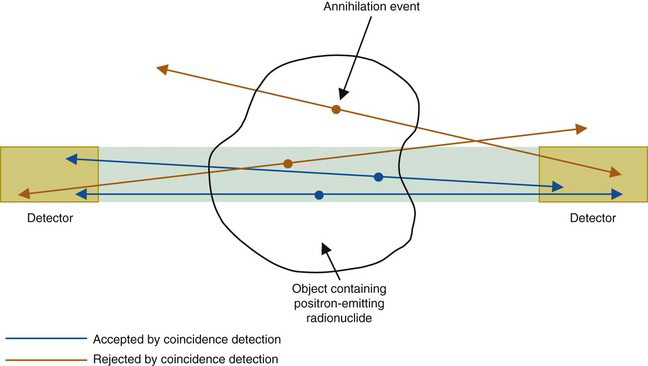
Coincidence logic (Chapter 8, Section F and Fig. 8-15) is employed to analyze the signals from the opposing detectors. For many PET scanners, this is accomplished by having the electronics attach a digital “time stamp” to the record for each detected event. Typically, this is done with a precision of approximately 1 or 2 nanoseconds (1 nsec = 10⁻⁹ sec). The coincidence processor examines the time stamp for each event in comparison with events recorded in the opposing detectors. A coincidence event is assumed to have occurred when a pair of events are recorded within a specified coincidence timing window, which typically is 6 to 12 nanoseconds.

Although annihilation photons are emitted simultaneously, a small but finite coincidence window width is needed to allow for differences in signal transit times through the cables and electronics, as well as different distances of travel by the two photons from the annihilation event to the detectors (see Section A.2). In addition, the detectors in a PET scanner do not have perfect timing precision and therefore have a finite timing resolution. Uncertainties that govern the timing resolution can arise from the statistical nature of the signal (which is produced by the conversion of 511-keV photons into light, electrons, or electron-hole pairs in the detector) and from electronic noise in the detector and associated circuits. Uncertainties also can arise from the electronic method used to determine the time at which the interaction occurred (see Chapter 8, Section F). For a pair of similar detectors, the timing uncertainties typically are well described by a gaussian distribution, and the timing resolution is defined as the full width at half maximum (FWHM) of this distribution. For scintillation detectors, the timing uncertainty is reduced, and the timing resolution improved, by using brighter and faster scintillators that produce a large number of light photons over a short time interval immediately after an interaction occurs. Timing resolution is typically in the range of 0.5 to 5 nsec, depending on which scintillator and photodetector is used.

The need for a finite window width permits other types of events to occur in coincidence, as discussed in Section A.9. Also, as discussed in Section A.4, the annihilation photons are not always emitted in precise back-to-back directions. The effects of these deviations from the ideal are discussed in the sections indicated.

The ability of ACD to localize events on the basis of coincidence timing, without the need for absorptive collimation, is referred to as electronic collimation. As was discussed in Chapter 14, Section C, the lead septa in standard parallel-hole collimators, which are necessary to obtain adequate spatial localization, also are responsible for the relatively low sensitivity of these collimators. Because ACD does not require a collimator to define spatial location, its sensitivity (number of events detected per unit of activity in the object) is much higher than is obtainable with the absorptive collimators used for conventional planar imaging and for SPECT. For comparable midplane resolution, the sensitivity of PET is many times higher than for SPECT.

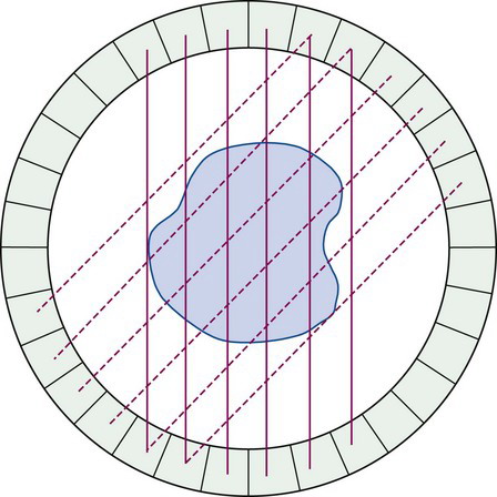
In addition, by incorporating multiple opposing detectors in a complete ring or other geometric array around the patient, and operating each detector in the array in coincidence with multiple detectors on the other side of the array, data for multiple projection angles can be acquired simultaneously (Fig. 18-2). Indeed, with a stationary ring or geometric array that completely surrounds the patient, it is possible to acquire data for all projection angles simultaneously. This allows the performance of relatively fast dynamic studies and the reduction of artifacts caused by patient motion.

FIGURE 18-2 Array of detectors operating in electronic coincidence with detectors on the opposite side of the ring. This allows simultaneous acquisition of projection views from many different angles. Solid and dotted lines illustrate two simultaneously acquired projection views.

2 Time-of-Flight PET

In theory, it is possible to determine the location along a line between the two ACD detectors at which the annihilation photons originated by determining the difference in the time at which they are detected by the two detectors. This technique, which would allow the formation of tomographic images without mathematical reconstruction algorithms, is called time-of-flight PET. If the difference in the arrival times of the photons is Δt, the location of the annihilation event, with respect to the midpoint between the two detectors, is given by

(18-1)

where c is the velocity of light (3 × 10¹⁰ cm /sec). According to this equation, to achieve 1-cm depth resolution would require timing resolution of approximately 66 picoseconds (1 psec = 10⁻¹² sec = 0.001 nsec). Although electronic circuits are capable of measuring this timing difference, the rise times of light output from scintillators currently available for PET imaging are too slow to provide this level of timing resolution. As well, the finite number of photoelectrons generated when an annihilation photon is detected gives rise to a “time jitter” during the rise time that adds to the uncertainty in event timing. This effect becomes more severe with detectors that have relatively low light output.

With the fastest available scintillators and careful design of electronic components and connections, it is possible to achieve timing accuracy at the level of a few hundred picoseconds. Although this is adequate to achieve localization only to within a few centimeters, images reconstructed from data acquired at this level of timing resolution have a higher signal-to-noise ratio than images reconstructed without time-of-flight information. This is because individual events can be constrained to lie within a smaller volume in the image reconstruction process. Figure 18-3 illustrates how the backprojection of data along one particular line of response is constrained to a smaller region of the reconstructed image matrix by the addition of time-of-flight information. To provide practically useful levels of time-of-flight information, only the fastest and brightest scintillators, such as LSO and LaBr₃, can be used (see Tables 7-2 and 18-2). Several commercially built systems incorporate some level of time-of-flight information using these materials. Although there are scintillators with even faster decay components, such as BaF₂, these are not favored because the signal-to-noise improvements that can be realized from time-of-flight information is typically more than offset by their lower density and therefore lower efficiency for detecting 511-keV annihilation photons.

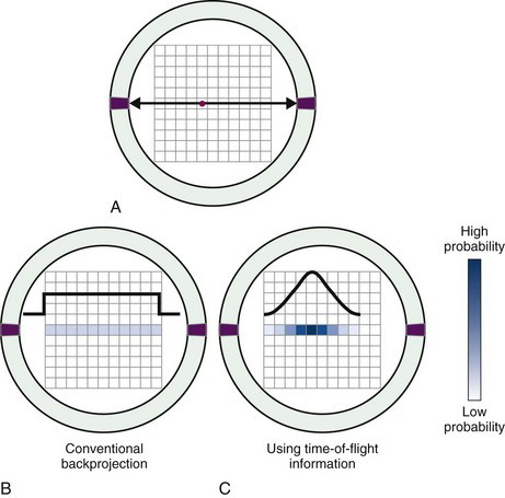
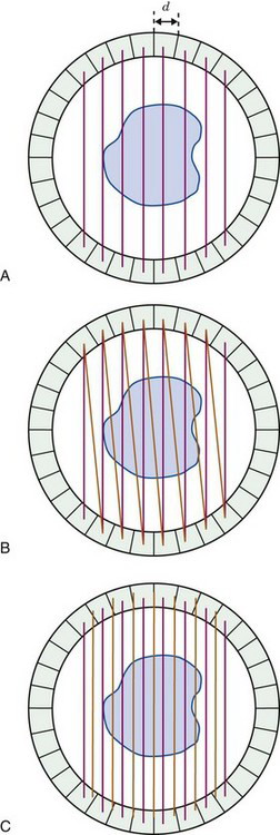
FIGURE 18-3 A, A pair of annihilation photons are emitted from a source (red dot) and detected in coincidence by opposing detectors. B, In the absence of time-of-flight information, there is no information about the location of the source along the line joining the two detectors. During reconstruction, the event is backprojected with equal probability of having occurred in all pixels along that line. C, With time-of-flight information, some limited localization of the event is possible and events are backprojected with probabilities that follow a Gaussian distribution, centered on pixel Δd (Equation 18-1) from the center of the scanner and with a full width at half maximum equal to the timing resolution of the detector pair.

3 Spatial Resolution: Detectors

The spatial resolution of ACD with discrete detector elements is determined primarily by the size of the individual detector elements. As shown in Figure 18-4A, for elements of width d, a one-dimensional (1-D) slice through the ACD point-source response profile at midplane between the detector pair is a triangle. The detector resolution, R_det has a FWHM = d/2. As the source moves toward either detector, the response profile becomes trapezoidal, eventually becoming a box of width d at the face of either detector. Considering a 2-D detector with width d and height h, the ACD response profile becomes a 3-D function, which is a pyramid at midplane and a rectangular box of area d × h at the face of either detector. Between these extremes, it is the frustum of a pyramid with lower base size equal to the size of the detectors and upper base size increasing linearly from zero at midplane to the size of the detectors at their face.

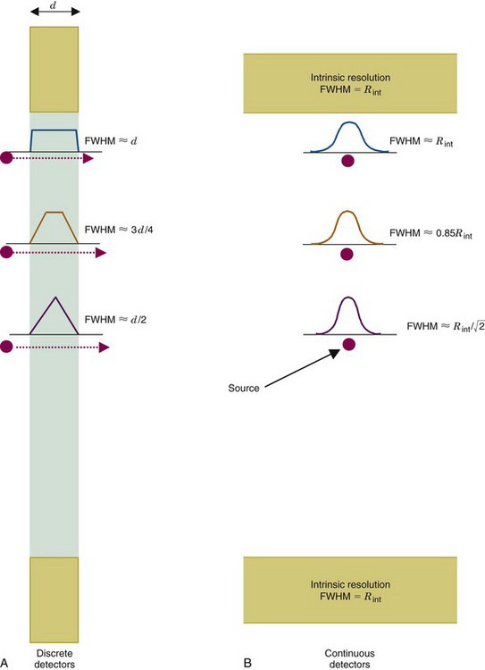
FIGURE 18-4 Spatial resolution of detector pair (R_det) for coincidence detection. A, For discrete detectors, spatial resolution is determined by the width of the detector element, d. At midplane, the coincidence response function is a triangle with full width at half maximum (FWHM) = d/2. As the source is moved closer to one of the detectors, the response function becomes trapezoidal in shape, eventually becoming a rectangle of width, d. B, For continuous detectors, spatial resolution is determined by the intrinsic resolution of the detector, R_int. At the midplane, the coincidence response function is approximately gaussian, with FWHM = R_int /. Near the face of a detector, it becomes FWHM = R_int.

Alternatively, consider an uncollimated pair of gamma camera detectors, also operating in coincidence mode (Fig. 18-4B). If their intrinsic spatial resolution (see Chapter 14, Section A.1) is a gaussian function with FWHM = R_int, then the spatial resolution of the detector pair for ACD also is a gaussian function with FWHM = R_int / at midplane. The ACD response profile becomes wider as the source moves toward either detector, with its FWHM eventually becoming equal to R_int at the face of either detector. Assuming that the resolution of the imaging detector is the same in all directions, the 2-D ACD response profile is obtained by rotating the 1-D gaussian function around its center.

For both discrete or gamma camera–type detectors, the spatial resolution of ACD varies by only approximately 30% in the central 60% of the space between the detectors (Fig. 18-5). By comparison, the resolution of a parallel-hole collimator can vary by several hundred percent over a comparable range (see Fig. 14-19). When profiles obtained from opposing views in SPECT are combined using the geometric mean, the variation in resolution within the space between the opposing detectors is reduced to a level comparable to ACD (see Fig. 17-8). The key difference is that the resolution of ACD is determined primarily by the size of the detector element or the intrinsic resolution of the camera detector, whereas for SPECT, the resolution is primarily determined by the collimator resolution at the midpoint between the two detectors. The latter is substantially degraded from its value at the face of the detector. This means that the collimator must have very high resolution at its face to achieve even moderately good resolution at midplane between the detectors. In turn, the requirement for high spatial resolution leads to relatively low detection efficiency with absorptive collimators (see Chapter 14, Section C). As discussed in Section A.8, this results in relatively low sensitivity for a SPECT system as compared with a PET system with comparable spatial resolution.

FIGURE 18-5 Measured line-spread functions for a pair of 17-mm-wide coincidence detectors as a function of source position between the two detectors. The detector separation was 42 cm. The FWHM varies by only 30% within the central 24 cm (57%) of the space between the two detectors.

(From Hoffman EJ, Huang S-C, Plummer D, Phelps ME: Quantitation in positron emission computed tomography: VI. Effect of nonuniform resolution. J Comput Assist Tomogr 6:987-999, 1982.)

4 Spatial Resolution: Positron Physics

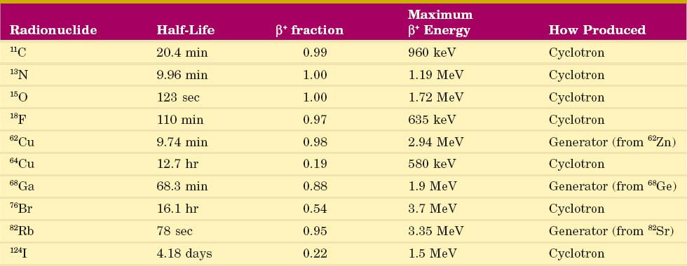
The spatial resolution of an ACD system is degraded from the values derived from simple geometry indicated in Figure 18-4 by two factors relating to the basic physics of positron emission and annihilation. The first is the finite range of positron travel before it undergoes annihilation. ACD defines the line along which the annihilation event took place, which is not precisely the location from which the decaying radioactive nucleus emitted the positron. The range of travel for a positron before it undergoes annihilation is essentially the same as the range of travel of an ordinary electron (or β particle) of similar energy (see Chapter 6, Section B.2). Figure 6-10 and Table 6-1 show the extrapolated range versus maximum energy for β particles, . The maximum energies of the positrons emitted from radionuclides used for nuclear medicine are in the range of 0.5 to 5 MeV (Table 18-1; see also Appendix C). Thus their extrapolated ranges are in the 0.1- to 2-cm range.

TABLE 18-1 SOME POSITRON-EMITTING NUCLIDES USED FOR IN VIVO IMAGING

The extrapolated range applies to the highest-energy positrons emitted by a radionuclide. However, positrons, like β particles, are emitted with a spectrum of energies. Only a small fraction have the full amount of energy available from the decay (see Fig. 3-2). In addition, the extrapolated range is the maximum distance that the electron would travel if it were not significantly deflected in any of its interactions and traveled in essentially a straight line to the end of its range. In reality, most electrons (and positrons) travel a tortuous path, often with multiple large-angle deflections (see Fig. 6-4). The result is that the average distance measured from the origin of the positrons to the end of their path is significantly smaller than their extrapolated range.

For purposes of defining the spatial resolution of ACD, the distance of interest is the effective positron range. This is the average distance from the emitting nucleus to the end of the positron range, measured perpendicular to a line defined by the direction of the annihilation photons (Fig. 18-6). This distance always is smaller than the extrapolated range for the positrons emitted by the radionuclide.

FIGURE 18-6 Blurring caused by positron range effects. The perpendicular distance from the decaying atom to the line defined by the two 511-keV annihilation photons is referred to as the effective positron range.

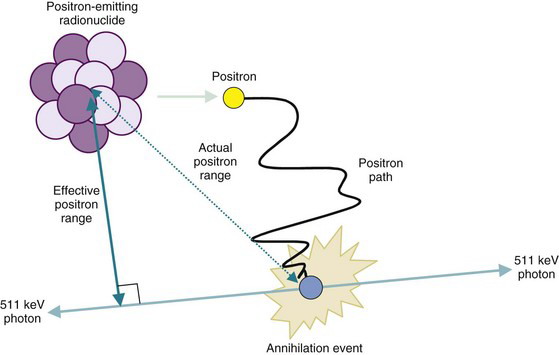
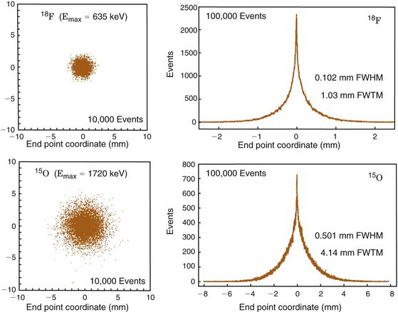
Figure 18-7 shows the positron range distribution for point sources of ¹⁸F ( = 0.635 MeV) and ¹⁵O ( = 1.72 MeV). According to Figure 6-10, the extrapolated ranges for these positrons in water would be approximately 2 mm and 8 mm, respectively; however, the FWHMs of their distribution profiles are only 0.1 mm and 0.5 mm.

FIGURE 18-7 Results of Monte Carlo simulations showing the distribution of annihilation sites for positron-emitting point sources in water for ¹⁸F ( = 0.635 MeV) and ¹⁵O ( = 1.72 MeV). The profile of the distribution is broader for ¹⁵O because of its higher average positron energy, which leads to a longer positron range prior to annihilation.

(From Levin CS, Hoffman EJ: Calculation of positron range and its effect on the fundamental limit of positron emission tomography system spatial resolution. Phys Med Biol 44:781-799, 1999.)

Note as well that the positron range distributions shown in Figure 18-7 have long tails and thus are not well described by gaussian functions. Therefore the FWHM is not the best indicator of the effect of positron range on ACD spatial resolution. Instead, the root mean square (rms) effective range often is used. Figure 18-8 shows the general relationship between rms effective range and maximum positron energy. Typical rms effective ranges (and thus the blurring caused by positron ranges) are on the order of 0.5 to 3 mm. Note that positron range is inversely proportional to the density of the absorber. Thus rms ranges would be proportionately higher in lung tissue and airways (ρ ~ 0.1-0.5 g/cm³) and lower in dense tissues such as bone (ρ ~ 1.3-2 g/cm³).

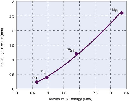
FIGURE 18-8 Root mean square range for positrons in water versus .

(Data from Derenzo SE: Mathematical removal of positron range blurring in high-resolution tomography. IEEE Trans Nucl Sci 33:565-569, 1986.)

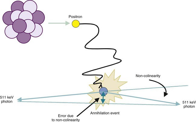
A second factor involving the physics of positrons is that the annihilation photons almost never are emitted at exactly 180-degree directions from each other (Fig. 18-9). This effect, which is due to small residual momentum of the positron when it reaches the end of its range, is known as noncolinearity. The angular distribution is approximately gaussian with FWHM approximately 0.5 degree. The effect on spatial resolution, expressed in terms of FWHM, is linearly dependent on the separation of the ACD detectors, D, and is given by

FIGURE 18-9 Noncolinearity of annihilation photons resulting from residual momentum of the electron and positron at annihilation. Noncolinearity leads to positioning errors. Angles are exaggerated in this example for purposes of illustration. Actual range of angles is about ±0.25 degree, centered at 180 degrees.

(18-2)

A typical value of D for a whole-body PET scanner is 80 cm. Thus the FWHM for blurring caused by noncolinearity is approximately 2 mm.

The system resolution of an ACD or PET detector system is obtained by combining the individual resolution components, in the same manner as the component resolutions are combined to determine the system resolution for a gamma camera system (see Chapter 14, Section C.4). Thus

(18-3)

where R_det is the spatial resolution of the detector system, as determined by the size of the discrete detector elements or the intrinsic resolution of continuous detectors (see Section A.3 and Fig. 18-4). For typical whole-body PET scanners, with either discrete detector elements or gamma camera detectors, the effects of positron range and noncolinearity combine to add anywhere from a few tenths of a millimeter to a few millimeters to system resolution.

Example 18-1

What fraction of PET system resolution at the center of the scanner bore is caused by positron range and noncolinearity blurring in the following three situations? (1) 6-mm-wide discrete detectors, separated by 80 cm, using ¹⁸F; (2) 2-mm-wide discrete detectors separated by 60 cm, using ⁶⁸Ga; (3) gamma camera detectors with 3-mm intrinsic resolution at 511 keV, separated by 60 cm, using ⁶⁸Ga.

Assume that the positron range distribution can be approximated by a gaussian function and use the rms effective range to represent the FWHM of that function.

Answer

For situation 1, the spatial resolution at the midpoint between 6-mm-wide discrete detectors is given by

The rms range for ¹⁸F is R_range ≈ 0.2 mm (see Fig. 18-8), and the noncolinearity for an 80-cm separation is

Using Equation 18-3, the system resolution is

Thus resolution blurring caused by positron range and noncolinearity for situation 1 adds approximately 17% to the system resolution, relative to the detector resolution.

For situation 2, using the same equations and Figure 18-8, the spatial resolution of 2-mm-wide discrete detectors is R_det = 1 mm, the rms range for ⁶⁸Ga is R_range ≈ 1.2 mm and the noncolinearity blurring for the 60-cm separation is 1.32 mm. Thus the system resolution is

In this situation, the additional blurring caused by positron range and noncolinearity approximately doubles the system resolution relative to detector resolution. Note that if ⁶⁸Ga is replaced by the lower-energy ¹⁸F in situation 2, the system resolution becomes ~1.7 mm, so the effects of positron range and noncolinearity still are substantial (~70%).

For situation 3, R_det = 3 / ≈ 2.12 mm (see Fig. 18-4) while other factors remain the same as in situation 2. Thus

Positron range and noncolinearity increase the system resolution by approximately 30% relative to detector resolution in this situation.

From Example 18-1, one can conclude that positron range and noncolinearity have a relatively small effect on system resolution for whole-body systems, which usually have larger detector elements (situation 1) or only moderately high spatial resolution (situation 3). This is especially true for ¹⁸F, the radionuclide most commonly used for clinical applications. However, their effects can be important limitations for high-resolution brain imaging or small-animal imaging devices (see Section B.5) that employ small discrete detector elements, especially for applications involving higher-energy positrons (situation 2).

Because they do not depend on technology, positron range and non colinearity create barriers for improving the spatial resolution of PET systems that cannot be overcome simply by using smaller detector elements. For example, independent of the detectors used, the blurring caused by noncolinearity will limit the achievable spatial resolution for a whole-body PET scanner to approximately 2 mm, because a bore size of 80-90 cm is required to accommodate the human body. Example 18-1 also demonstrates that when system resolution is dominated by one component, the gains achieved by improving other components of resolution may be small.

5 Spatial Resolution: Depth-of-Interaction Effect

A substantial thickness of scintillator material is required to efficiently stop 511-keV annihilation photons. In a gamma camera, typical NaI(Tl) detector crystal thicknesses are 1.25 cm or less. PET systems generally employ 2- to 3-cm-thick scintillators with greater stopping power, such as BGO or LSO. For PET systems using arrays of detectors in multiple coincidence mode around the object, the relatively thick detector elements lead to a degradation of resolution known as the depth of interaction (DOI) effect. Although the effect also occurs in the axial direction in scanners that use cross-plane coincidence detection for 3-D data acquisition (see Section C.2), the primary effect is in the radial direction, and the discussion focuses on this aspect of the problem.

Figure 18-10 illustrates the cause of the problem for a detector system that uses a circular array of elements, all or most elements of which operate in multicoincidence mode with other elements in the array. For a source located near the center of the scanner, spatial resolution is determined by the width of the detector element, R_det = d/2, as described in Section A.3 and illustrated in Figure 18-4. However, for a source located away from the center, the apparent width of the detector element becomes

FIGURE 18-10 Apparent width of a detector element, d′, increases with increasing radial offset in a PET scanner consisting of a circular array of detector elements. Because the depths at which the γ rays interact within the scintillation crystal are unknown, the annihilation event for a pair of photons recorded in coincidence could have occurred anywhere within the shaded volume. The magnitude of the effect depends on the source location, the diameter of the scanner, D, the length of the crystal elements, x, and the width of the detector elements, d.

(18-4)

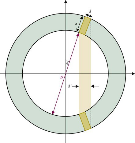
where d, x, and θ are as indicated in Figure 18-10. The apparent change in width results from the angulation between the detectors and from lack of knowledge about the depth at which an interaction has occurred within the detector crystal. The spatial resolution (FWHM) then becomes R′_det = d′/2. Using Equation 18-4, this can be written as

(18-5)

From this equation it can be seen that the DOI effect is described by a multiplicative factor applied to the value of detector resolution at the midpoint between a pair of directly opposed detectors.

Equation 18-5 is only an approximation because the thickness of detector material is not constant across the width of the detector element seen by the source. Note as well that, for thin detector elements [(x/d) << 1], it is possible that R′_det < R_det. The same would be true for a very efficient detector material (or a very thin detector) that would stop most of the annihilation photons in a thin layer at the entrance to the detector. However, these conditions never apply in practice. Typically, x ~ 2 to 3 cm and d ~ 0.3 to 0.6 cm. For a whole-body PET scanner with 4-mm-wide detectors on a diameter of 80 cm, the DOI effect causes approximately a 40% degradation of resolution at a distance of 10 cm from the center of the field of view (FOV).

The DOI effect is somewhat different for systems that use hexagonal or octagonal arrays as opposed to circular arrays of detector elements. With hexagonal or octagonal arrays, as the source moves away from the center of the scanner, some portion of an opposing array still remains perpendicular to it, at least over a distance comparable to the width of a segment of the array. Consequently, there is less variation in the DOI effect across the FOV. At the center of the FOV, the effect is somewhat larger than at the center for a circular array of the same diameter, whereas at the periphery it is somewhat smaller. On average, the DOI effect is comparable for both segmented and circular arrays.

Note also in Equations 18-4 and 18-5 that, for a given radial distance away from the center of the scanner, θ and sin θ become smaller (and thus R′_det becomes smaller) as the diameter of the detector ring becomes larger. Because of the DOI effect, PET scanners often are built with detector arrays that are of larger diameter than would be necessary to fit the patient, which in turn increases detector costs.

6 Spatial Resolution: Sampling

In ACD, the FWHM of the detector resolution is one-half the width of a detector element (see Fig. 18-4). For a stationary array of detector elements, each of width d, the sampling interval between parallel projection lines also is d (Fig. 18-11A). Considering only detector resolution, it can be shown that this leads to undersampling of object profiles, which in turn leads to a distortion of the high-frequency content (i.e., the fine details) of the reconstructed image (see Fig. 16-11 and Section C). According to Equation 16-14, three samples should be acquired per FWHM of spatial resolution. In theory, this would translate into a requirement for six samples over an interval equal to the width of a detector element. However, as described elsewhere in this section, system resolution is degraded from the theoretical limits established by intrinsic resolution by other factors, so that coarser sampling is acceptable. Nonetheless, some additional sampling is required beyond that illustrated in Figure 18-11A.

FIGURE 18-11 A, For a stationary array of discrete detector elements, the linear sampling distance is the same as the detector element width, d, which is insufficient to support the resolution of the detectors (~d/2). B, Linear sampling distance is reduced to d/2 when coincidences with immediately adjacent detectors are allowed. C, For image reconstruction, these samples are treated as if they came from a set of virtual detectors offset by half the detector width relative to the actual detectors.

In practice, two samples usually are acquired per detector element width. Although less than the theoretical ideal, this results in little noticeable distortion of clinical images. Some earlier scanners actually incorporated a mechanical shift to acquire two sets of data with the detector elements shifted by half the width of a detector element between acquisitions. This approach was mechanically cumbersome. The modern approach is to use coincidence events in adjacent pairs of detector elements, thereby creating additional samples between the detector elements, as illustrated in Figure 18-11B. These are treated as samples acquired with a virtual set of detectors located between the actual detector elements, as shown in Figure 18-11C. The ray paths for the additional samples are not quite parallel to those for directly opposed detectors, but this seems to have little effect on the reconstructed image across most of the useful FOV.

Note that combining data for adjacent pairs of detectors into a single projection view as illustrated in Figure 18-11B and C, reduces the number of projection angles available from a stationary ring of detectors by half. Note also that PET systems that use continuous (i.e., gamma camera type) detectors (see Section B.3) can use arbitrarily chosen sampling intervals and thus can avoid some of the sampling problems associated with discrete detector arrays.

7 Spatial Resolution: Reconstruction Filters

The discussions in the preceding sections describe the spatial resolution achievable with PET systems, as determined by the physical characteristics of the imaging device and the basic physics of positron decay. However, as discussed in Chapter 16, Sections B.3 and C.3, spatial filters are applied to the recorded projection profiles to suppress noise in the reconstructed image (see Fig. 16-12). Inevitably, this results in some degradation of spatial resolution. In general, the fewer the number of counts recorded in an image, the lower the filter cut-off frequency (k_cut-off) and the greater the loss of spatial resolution.

The selection of cut-off frequency depends in part on the type of study. Thus a brain scan might be reconstructed with a cut-off frequency yielding 6-mm spatial resolution, whereas an abdominal scan, with more tissue attenuation and generally lower count densities, might be reconstructed with a filter yielding 10-mm spatial resolution. As well, the sensitivity (number of counts recorded per unit of activity in the patient) affects the statistical quality of the image and the degree of spatial filtering required to achieve an acceptable noise level in the image. As discussed in the following section and in Section B, PET systems, especially those employing multiple detector rings and multi-ring coincidence detection, have substantially higher detection efficiencies (by orders of magnitude) than is achievable with typical SPECT systems. Thus PET images usually can be reconstructed with higher cut-off frequencies, and their final spatial resolution generally is superior to SPECT images.

8 Sensitivity

The sensitivity of PET, like that of all imaging devices, is determined primarily by the absorption efficiency of the detector system and its solid angle of coverage of the imaged object. The true coincidence rate, R_true, for a positron-emitting source located in an absorbing medium between a pair of coincidence detectors is given by

(18-6)

where E is the source emission rate (positrons/sec); ε is the intrinsic efficiency of each detector, that is, the fraction of incident photons detected (Equation 11-9, assumed to be the same for both detectors); and µ and T are the linear attenuation coefficient and total thickness of the object, respectively. g_ACD is the geometric efficiency of the detector pair, that is, the fraction of annihilation events in which both photons are emitted in a direction to be intercepted by the detectors.

As shown in Figure 18-4, the shape as well as the amplitude of the point-source response profile (i.e., g_ACD for a point source) varies with the location of the source between the two detectors. In one dimension, the profile is triangular at the midpoint between the detectors, rectangular at the face of either detector, and trapezoidal at locations between. In two dimensions, the ACD response at the midpoint is a pyramid, whereas at the surface of either of the detectors it is a rectangular box. At points between, it is the frustum of a pyramid. In all cases, the lower base is equal to the area of the detectors.

Maximum geometric efficiency for ACD is obtained for a point source located precisely at the midpoint of the centerline between the two detectors. However, as illustrated in Figure 18-4, this value does not apply when the point source is moved even slightly away from the centerline, or from the midpoint of that line. Thus a more appropriate measure for distributed sources is the average geometric efficiency within the sensitive volume for ACD. Midway between the two detectors, this is given by

(18-7)

where D is the distance between the detectors and A_det is the area of the detector facing the source.

The term in brackets in Equation 18-7 is the geometric efficiency for a single detector for a point source located at the midpoint of the centerline between the detectors. (As discussed in Chapter 11, Section A.2, this expression is valid when the detector dimensions are “small” in comparison with the source-to-detector distance.) The factor of 2 accounts for the fact that two detectors are used and that if one photon is emitted in a proper direction toward one detector, the other photon is virtually assured of being emitted in the proper direction toward the other. The factor of 1/3 is the average geometric efficiency across the sensitive volume at midplane, that is, the average height of a pyramid.

Actual PET systems typically employ many small detector elements arranged in circular, hexagonal, or octagonal arrays. Each detector element is operated in coincidence with many detectors on the opposing side of the ring, as shown in Figure 18-12. This multicoincidence operation has useful and important consequences for both the magnitude and uniformity of geometric efficiency.

Related posts:

Digital Image Processing in Nuclear Medicine The Gamma Camera: Basic Principles Electronic Instrumentation for Radiation Detection Systems Counting Systems Problems in Radiation Detection and Measurement Decay of Radioactivity

Stay updated, free articles. Join our Telegram channel

Join