chapter 11 Problems in Radiation Detection and Measurement

Nuclear medicine studies are performed with a variety of types of radiation measurement instruments, depending on the kind of radiation source that is being measured and the type of information sought. For example, some instruments are designed for in vitro measurements on blood samples, urine specimens, and so forth. Others are designed for in vivo measurements of radioactivity in patients (Chapter 12). Still others are used to obtain images of radioactive distributions in patients (Chapters 13, 14, and 17–19).

All these instruments have special design characteristics to optimize them for their specific tasks, as described in the chapters indicated above; however, some considerations of design characteristics and performance limitations are common to all of them. An important consideration for any radiation measurement instrument is its detection efficiency. Maximum detection efficiency is desirable because one thus obtains maximum information with a minimum amount of radioactivity.

Also important are the instrument’s counting rate limitations. There are finite counting rate limits for all counting and imaging instruments used in nuclear medicine, above which inaccurate results are obtained because of data losses and other data distortions. Nonpenetrating radiations, such as β particles, have special detection and measurement problems. In this chapter, we discuss some of these general considerations in nuclear medicine instrumentation.

A Detection Efficiency

1 Components of Detection Efficiency

Detection efficiency refers to the efficiency with which a radiation-measuring instrument converts emissions from the radiation source into useful signals from the detector. Thus if a γ-ray-emitting source of activity A (Bq) emits η γ rays per disintegration, the emission rate ξ of that source is

(11-1)

If the counting rate recorded from this source is R [counts per second (cps)], then the detection efficiency D for the measuring system is

(11-2)

Alternatively, if the emission rate ξ and detection efficiency D are known, one can estimate the counting rate that will be recorded from the source from

(11-3)

In general, it is desirable to have as large a detection efficiency as possible, so that a maximum counting rate can be obtained from a minimum amount of activity. Detection efficiency is affected by several factors, including the following:

1 The geometric efficiency, which is the efficiency with which the detector intercepts radiation emitted from the source. This is determined mostly by detector size and the distance from the source to the detector.

2 The intrinsic efficiency of the detector, which refers to the efficiency with which the detector absorbs incident radiation events and converts them into potentially usable detector output signals. This is primarily a function of detector thickness and composition and of the type and energy of the radiation to be detected.

3 The fraction of output signals produced by the detector that are recorded by the counting system. This is an important factor in energy-selective counting, in which a pulse-height analyzer is used to select for counting only those detector output signals within a desired amplitude (energy) range.

4 Absorption and scatter of radiation within the source itself, or by material between the source and the radiation detector. This is especially important for in vivo studies, in which the source activity generally is at some depth within the patient.

In theory, one therefore can describe detection efficiency D as a product of individual factors,

(11-4)

where g is the geometric efficiency of the detector, ε is its intrinsic efficiency, f is the fraction of output signals from the detector that falls within the pulse-height analyzer window, and F is a factor for absorption and scatter occurring within the source or between the source and detector. Each of these factors are considered in greater detail in this section. Most of the discussion is related to the detection of γ rays with NaI(Tl) detector systems. Basic equations are presented for somewhat idealized conditions. Complications that arise when the idealized conditions are not met also are discussed. An additional factor applicable for radionuclide imaging instruments is the collimator efficiency, that is, the efficiency with which the collimator transmits radiation to the detector. This is discussed in Chapter 13.

2 Geometric Efficiency

Radiation from a radioactive source is emitted isotropically, that is, with equal intensity in all directions. At a distance r from a point source of γ-ray-emitting radioactivity, the emitted radiation passes through the surface of an imaginary sphere having a surface area 4π r². Thus the flux I of radiation passing through the sphere per unit of surface area, in units of γ rays/sec/cm², is

(11-5)

where ξ is the emission rate of the source and r is given in centimeters. As distance r increases, the flux of radiation decreases as 1/r² (Fig. 11-1). This behavior is known as the inverse-square law. It has important implications for detection efficiency as well as for radiation safety considerations (see Chapter 23). The inverse-square law applies to all types of radioactive emissions.

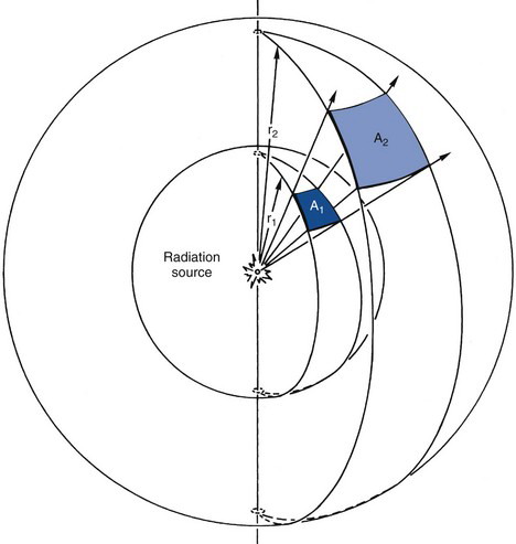
FIGURE 11-1 Illustration of the inverse-square law. As the distance from the radiation source increases from r₁ to r₂, the radiations passing through A₁ are spread out over a larger area A₂. Because A α r², the intensity of radiation per unit area decreases as 1/r².

The inverse-square law can be used to obtain a first approximation for the geometric efficiency of a detector. As illustrated in Figure 11-1, a detector with surface area A placed at a distance r from a point source of radiation and facing toward the source will intercept a fraction A/4πr² of the emitted radiation. Thus its geometric efficiency g_p is

(11-6)

where the subscript p denotes a point source. The approximation sign indicates that the equation is valid only when the distance from the point source to the detector is large in comparison with detector size, as discussed in the following paragraphs.

Example 11-1

Calculate the geometric efficiency for a detector of diameter d = 7.5 cm at a distance r = 20 cm from a point source.

Answer

The area, A, of the detector is

Therefore, from Equation 11-6,

Thus the detector described in Example 11-1 intercepts less than 1% of the emitted radiation and has a rather small geometric efficiency, in spite of its relatively large diameter. At twice the distance (40 cm), the geometric efficiency is smaller by another factor of 4.

Equation 11-6 becomes inaccurate when the source is “close” to the detector. For example, for a source at r = 0, it predicts g_p = ∞. An equation that is more accurate at close distances for point sources located on the central axis of a circular detector is

(11-7)

where θ is the angle subtended between the center and edge of the detector from the source (Fig. 11-2). For example, when the radiation source is in contact with the surface of a circular detector, θ = 90 degrees and g_p = 1/2 (Fig. 11-3A).

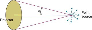
FIGURE 11-2 Point-source geometric efficiency for a circular large-area detector placed relatively close to the source depends on the angle subtended, θ (Equation 11–7).

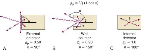
FIGURE 11-3 Examples of point-source geometric efficiencies computed from Equation 11-7 for different source-detector geometries.

Geometric efficiency can be increased by making θ even larger. For example, at the bottom of the well in a standard well counter (Chapter 12, Section A.2) the source is partially surrounded by the detector (Fig. 11-3B) so that θ ≈ 150 degrees and g_p ≈ 0.93. In a liquid scintillation counter (see Chapter 12, Section C), the source is immersed in the detector material (scintillator fluid), so that θ = 180 degrees and g_p = 1 (Fig. 11-3C).

Equation 11-7 avoids the obvious inaccuracies of Equation 11-6 for sources placed close to the detector; however, even Equation 11-7 has limitations when the attenuation by the detector is significantly less than 100%. This problem is discussed further in Section A.5.

The approximations given by Equations 11-6 and 11-7 apply to point sources of radiation located on the central axis of the detector. They also are valid for distributed sources having dimensions that are small in comparison to the source-to-detector distance; however, for larger sources (e.g., source diameter 0.3r) more complex forms are required.¹

3 Intrinsic Efficiency

The fraction of radiation striking the detector that interacts with it is called the intrinsic efficiency ε of the detector:

(11-8)

Intrinsic efficiency ranges between 0 and 1 and depends on the type and energy of the radiation and on the attenuation coefficient and thickness of the detector. For a point source located on the central axis of a γ-ray detector, it is given by

(11-9)

where µ_l (E) is the linear attenuation coefficient of the detector at the γ-ray energy of interest, E, and x is the detector thickness. In Equation 11-9 it is assumed that any interaction of the γ ray in the detector produces a potentially useful signal from the detector, although not necessarily all are recorded if energy-selective counting is used, as described in Section A.4.

The mass attenuation coefficient µ_m versus E for NaI(Tl) is shown in Figure 6-17. Numerical values are tabulated in Appendix D. Values of µ_l for Equation 11-9 may be obtained by multiplication of µ_m by 3.67 g/cm³, the density of NaI(Tl). Figure 11-4 shows intrinsic efficiency versus γ-ray energy for NaI(Tl) detectors of different thicknesses. For energies below approximately 100 keV, intrinsic efficiency is near unity for NaI(Tl) thicknesses greater than approximately 0.5 cm. For greater energies, crystal thickness effects become significant, but a 5-cm-thick crystal provides ε > 0.8 over most of the energy range of interest in nuclear medicine.

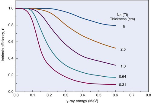
FIGURE 11-4 Intrinsic efficiency versus γ-ray energy for NaI(Tl) detectors of different thicknesses.

The intrinsic efficiency of semiconductor detectors also is energy dependent. Because of its low atomic number, silicon (Si, Z=14) is used primarily for low-energy γ rays and x rays (100 keV), whereas germanium (Ge, Z=32) is preferred for higher energies. The effective atomic number of NaI(Tl) is approximately 50 (Table 7-2), which is greater than either Ge or Si; however, comparison with Ge is complicated by the fact that Ge has a greater density than NaI(Tl) (ρ = 5.68 g/cm³ vs. 3.67 g/cm³). The linear attenuation coefficient of NaI(Tl) is greater than that of Ge for E 250 keV, but at greater energies the opposite is true; however, differences in cost and available physical sizes favor NaI(Tl) over Ge or Si detectors for most applications. The effective atomic numbers of cadmium telluride (CdTe) and cadmium zinc telluride (CZT) detectors are similar to that of NaI(Tl) (see Tables 7-1 and 7-2). They also have higher densities (ρ ≈ 6 g/cm³). Thus for detectors of similar thickness, these detectors have somewhat greater intrinsic detection efficiencies than Na(Tl).

Gas-filled detectors generally have reasonably good intrinsic efficiencies (ε ≈ 1) for particle radiations (β or α) but not for γ and x rays. Linear attenuation coefficients for most gases are quite small because of their low densities (e.g., ρ ≈ 0.0013 g/cm³ for air). In fact, most gas-filled detectors detect γ rays primarily by the electrons they knock loose from the walls of the detector into the gas volume rather than by direct interaction of γ and x rays with the gas. Intrinsic efficiencies for Geiger-Müller (GM) tubes, proportional counters, and ionization chambers for γ rays are typically 0.01 (1%) or less over most of the nuclear medicine energy range. Some special types of proportional counters, employing xenon gas at high pressures or lead or leaded glass γ-ray converters,* achieve greater efficiencies, but they still are generally most useful for γ- and x-ray energies below approximately 100 keV.

4 Energy-Selective Counting

The intrinsic efficiency computed from Equation 11-9 for a γ-ray detector assumes that all γ rays that interact with the detector produce an output signal; however, not all output signals are counted if a pulse-height analyzer is used for energy-selective counting. For example, if counting is restricted to the photopeak, most of the γ rays interacting with the detector by Compton scattering are not counted.

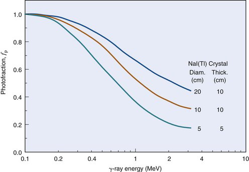
The fraction of detected γ rays that produce output signals within the pulse-height analyzer window is denoted by f. The fraction within the photopeak is called the photofraction f_p. The photofraction depends on the detector material and on the γ-ray energy, both of which affect the probability of photoelectric absorption by the detector. It depends also on crystal size (see Fig. 10-8) because with a larger-volume detector there is a greater probability of a second interaction to absorb the scattered γ ray following a Compton-scattering interaction in the detector (or of annihilation photons following pair production). Figure 11-5 shows the photofraction versus energy for NaI(Tl) detectors of different sizes.

FIGURE 11-5 Photofraction versus γ-ray energy for cylindrical NaI(Tl) detectors of different sizes.

If energy-selective counting is not used, then f ≈ 1 is obtained. (Generally, some energy discrimination is used to reject very small amplitude noise pulses.) Full-spectrum counting provides the maximum possible counting rate and is used to advantage when a single radionuclide is counted, with little or no interference from scattered radiation. This applies, for example, to many in vitro measurements (see Chapter 12).

5 Some Complicating Factors

a Nonuniform Detection Efficiency

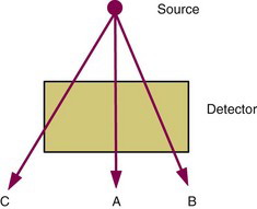
Equations 11-6, 11-7, and 11-9 are somewhat idealized in that they assume that radiation is detected with uniform efficiency across the entire surface of the detector. In some cases, this assumption may be invalid. Figure 11-6 shows some examples for different trajectories from a point source of radiation. For trajectory A, the thickness of detector encountered by the radiation and employed for the calculation of intrinsic efficiency in Equation 11-9 conforms to what normally would be defined as the “detector thickness” in that equation. However, for trajectory B, a greater thickness is encountered and the intrinsic efficiency is larger. On the other hand, for trajectory C, near the edge of the detector, a smaller thickness of detector material is encountered and the intrinsic efficiency is smaller. Partial penetration of the beam for trajectory C sometimes is called an edge effect.

FIGURE 11-6 Three possible trajectories for radiations striking a detector from a point source, each having a different intrinsic detection efficiency.

Thus, unless the attenuation by the detector is “very high” (essentially 100% within a thin layer near the surface), the intrinsic efficiency will vary across the surface of the detector. As well, the detector diameter (or area) used for the calculation of geometric efficiency in Equation 11-6 or 11-7 becomes ill-defined when edge effects are significant. When the complications illustrated in Figure 11-6 are significant, detection efficiency must be calculated by methods of integral calculus, rather than with the simplified equations described thus far. The calculations are complex and a complete analysis is beyond the scope of this text, but they have been analyzed in other books.² A few practical implications derived from more advanced calculations are presented here.

The nonuniform attenuation illustrated in Figure 11-6 affects both geometric efficiency (edge effects) and intrinsic efficiency. The parameter that accounts for both of these quantities is the total detection efficiency, ε_t. When idealized conditions apply, this can be obtained simply by multiplying the result of Equation 11-6 or 11-7 by the result from Equation 11-9

(11-10)

It is reasonable to use Equation 11-10 to compute total detection efficiency if the resulting discrepancy from a more exact calculation is “small,” for example, less than 10%. If the discrepancy is larger, then one must consider using the more complex methods of integral calculus.

Figure 11-7 shows three detector profiles with different levels of effect for the trajectories shown in Figure 11-6. As compared with a “box” profile (i.e., one with equal thickness and width), a “wide” profile presents a greater range of potential detector thicknesses (trajectory B in Fig. 11-6

Only gold members can continue reading. Log In or Register to continue