Fig. 8.1
Texture analysis of gadoxetic acid-enhanced MR images in patient with chronic liver disease. This figure shows differences in the GLCM according to the severity of liver fibrosis. Second-order descriptors derived from this matrix can offer quantitative information relevant for the assessment of liver fibrosis
The dissimilarity expresses the same characteristic than the contrast, but the weights of inputs of the GCLM increase linearly from the diagonal rather than quadratically for the contrast. These two descriptors are thus often correlated.
The entropy (randomness of the matrix) relies to the spreading of the GCLM diagonal. The entropy is the inverse of energy. These parameters are often correlated.
The homogeneity (uniformity of co-occurrence matrix) inversely evolves with the contrast. Homogeneity is high when the differences between co-occurrences are small. It is more sensitive on the diagonal elements of the GCLM than the contrast which depends on elements outside the diagonal.
The correlation may be described as a measurement of the linear dependency of gray levels of the image. The cluster shade and cluster prominence give information about the degree of symmetry of the GCLM. High values represent low symmetric pattern.
The main difficulty when using GCLM is to fix the parameters because this step needs to be performed case by case. The distance d must reflect the local correlation between the pixels. It is admitted that the correlation is more pertinent for short distances and, typically, d is fixed equal to 1. In practice, GCLM is computed over four orientations (i.e., 0°, 45°, 90°, and 135°) according to Haralick recommendations [29]. The features are computed for each orientation and can be concatenated in a single array of descriptors or averaged to obtain an array of descriptors invariant regarding to the rotation. The choice of the window (i.e., the number of gray levels in the parametric image) is also important and imposes a compromise between the pertinence of the descriptors and the fidelity of the texture.
Another method to derive second-order statistics is the gray-level run-length matrix (GLRLM). A gray-level run is defined as the length in number of pixels of consecutive pixels that have the same gray-level value. From the GLRLM, features can be extracted describing short- and long-run emphasis, gray-level nonuniformity, run-length nonuniformity, run percentage, low gray-level run emphasis, and high gray-level run emphasis [1, 28]. The short-run emphasis characterizes the smoothness of the texture, whereas the long-run emphasis characterizes the coarseness. The run percentage is the ratio between the number of runs over the number of pixels in the image. It characterizes the homogeneity of the texture. The gray-level nonuniformity measures the uniformity of run distribution. It is minimal when the runs are uniformly distributed between the gray levels. The run-length nonuniformity measures the uniformity of run length and increases with the number of runs of same length.
Other matrices have been proposed to characterize the texture in the spatial domain such as the gray-level size zone matrix (GLSZM). GLSZM does not require computation in several directions, in contrast to GLRLM and GLCM. However, the degree of gray-level quantization has an important impact on the texture classification performance. Similarly to GLRLM, descriptors can be derived from the analysis of this matrix such as the small-zone size emphasis, large-zone size emphasis, low gray-level zone emphasis, high gray-level zone emphasis, small-zone low-gray emphasis, small-zone high-gray emphasis, large-zone low-gray emphasis, large-zone high-gray emphasis, gray-level nonuniformity, zone size nonuniformity, and zone size percentage [30].
8.5.3 Analysis Based on the Organization of Geometric Pattern in the Image Domain
Filter grids can be applied on the images to extract repetitive or non-repetitive patterns. These methods include fractal analysis, wherein patterns are imposed on the images and the number of grid elements containing voxels of a specified value is computed; Minkowski functionals, which assess patterns of voxels whose intensity is above a threshold [31]; and Laplacian transforms of Gaussian band-pass filters that extract areas with increasingly coarse texture patterns from the images [32].
8.5.4 Texture Analysis in the Frequency Domain
These methods use filtering tools such as the Fourier transform, the wavelet decomposition, and the Gabor filter to extract the information. The 2D Fourier transform allows to represent the frequency spectrum on images in which each coefficient corresponds to a frequency in a given orientation. Therefore, the center of the spectra includes the low frequencies and the extremities the high frequencies. An image with a smooth texture will display a spectrum with high values concentrated close to the center, whereas an image with a rough texture will display a spectra with high value concentrated at the extremities. Quantitative information related to the texture can be extracted by decomposing the spectra into sub-bands according to their polar coordinates and calculating the average, energy, variance, and maximum [33]. The Fourier transform can also be applied in local neighbors in the image. It is possible to determine a radial spectrum on windows with increasing size by averaging the coefficient of the Fourier spectrum over all orientations. A principal component analysis is performed to identify the range of frequencies and the size window explaining the variability [34]. The Fourier spectrum only contains frequency information.
In contrast, Gabor filters and the wavelet transforms provide both frequency and spatial information. Gabor filters have the ability to model the direction and frequency sensitivity by decomposing the image spectrum in a narrow range of frequencies and orientations. In the spatial domain, the Gabor filter is a Gaussian function modulated by a complex sinusoid and a Gaussian surface centered on a central frequency F with an orientation θ in the frequency domain. A conventional practice with Gabor filters consists in using filter banks, each centered on a different central frequency and orientation, by covering the whole frequency domain. Each pixel gives a response for each filter. To have a different proportion covered by each filter and to limit the overlap, thus the redundancy of information, Manjunath and Ma have proposed to decompose the spectrum in several scales and orientations [35]. Mean and standard deviation of the filter responses are calculated to extract the texture signature.
Nevertheless, due to the non-orthogonality of Gabor filters, texture attributes derived from these filters can be correlated. It is difficult to determine if a similarity observed between the analysis scales is linked to the property of the image or to redundancy in the information. Thus for each scale of application, parameters defining the filter must be modified.
This issue is addressed by the use of wavelets, offering a uniform analysis framework by decomposing the image into orthogonal and independent sub-bands. Briefly, the wavelet decomposes the image with a series of functions obtained by translation and scaling from an initial function, called mother wavelet. Wavelet decomposition of an image is the convolution product between the image and the wavelet functions [31].
8.6 Data Reduction
The number of descriptive image features can approach the complexity of data obtained with gene expression profiling. With such large complexity, there is a danger of overfitting analyses, and hence, dimensionality must be reduced by prioritizing the features. Dimensionality reduction can be divided into feature extraction and feature selection. Feature extraction transforms the data in the high-dimensional space to a space of fewer dimensions, as in principal component analysis.
Feature selection techniques can be broadly grouped into approaches that are classifier dependent (wrapper and embedded methods) and classifier independent (filter methods). Wrapper methods search the space of feature subsets, using the training/validation accuracy of a particular classifier as the measure of utility for a candidate subset. This may deliver significant advantages in generalization, though has the disadvantage of a considerable computational expense, and may produce subsets that are overly specific to the classifier used. As a result, any change in the learning model is likely to render the feature set suboptimal. Embedded methods exploit the structure of specific classes of learning models to guide the feature selection process. These methods are less computationally expensive, and less prone to overfitting than wrappers, but still use quite strict model structure assumptions.
In contrast, filter methods evaluate statistics of the data independently of any particular classifier, thereby extracting features that are generic, having incorporated few assumptions. Each of these three approaches has its advantages and disadvantages, the primary distinguishing factors being speed of computation, and the chance of overfitting. In general, in terms of speed, filters are faster than embedded methods which are in turn faster than wrappers. In terms of overfitting, wrappers have higher learning capacity so are more likely to overfit than embedded methods, which in turn are more likely to overfit than filter methods.
A primary advantage of filters is that they are relatively cheap in terms of computational expense and are generally more amenable to a theoretical analysis of their design. The defining component of a filter method is the relevance index quantifying the utility of including a particular feature in the set. The filter-based feature selection methods can be divided into two categories: univariate methods and multivariate methods. In case of univariate methods, the scoring criterion only considers the relevancy of features ignoring the feature redundancy, whereas multivariate methods investigate the multivariate interaction within features, and the scoring criterion is a weighted sum of feature relevancy and redundancy [36–38].
One of the simplest methods relies on the computation of cross correlation matrices, whereby the correlation between each pair of features is computed (Fig. 8.2). The resulting matrix is subsequently thresholded to identify subsets of features that are highly correlated.


Fig. 8.2
Illustration of the feature selection process. The cross correlation matrix on the left is reordered with linkage algorithms on the right and thresholded to a given value of correlation coefficient. For data analysis, one feature of each group on the right can be selected based on maximum relevancy, e.g., maximum patient interpatient variability
A single feature from each subset can then be selected based on maximum relevancy.
8.7 Data Classification
For data mining, unsupervised and supervised analysis options are available. The distinction in these approaches is that unsupervised analysis does not use any outcome variable, but rather provides summary information and graphical representations of the data. Supervised analysis, in contrast, creates models that attempt to separate or predict the data with respect to an outcome or phenotype.
Clustering is the grouping of like data and is one of the most common unsupervised analysis approaches. There are many different types of clustering. Hierarchical clustering, or the assignment of examples into clusters at different levels of similarity into a hierarchy of clusters, is a common type. Similarity is based on correlation (or Euclidean distance) between individual examples or clusters.
Alternatively, k-means clustering is based on minimizing the clustering error criterion which for each point computes its squared distance from the corresponding cluster center and then takes the sum of these distances for all points in the data set.
The data from this type of analyses can be graphically represented using the cluster color map. Cluster relationships are indicated by treelike structures adjacent to the color map or by k-means cluster groups [24, 39] (Fig. 8.3).


Fig. 8.3
Graphical representation of a radiomics data set. Each patient represents a row of the matrix (np, number of patients), and each column represents one of the features (nf, number of features). First-order imaging parameters based on MR elastography data acquired at several mechanical frequencies in patients with liver cirrhosis and portal hypertension. The hierarchical cluster relationships are indicated by treelike structures on the right of the matrix representation. Alternatively, clustering by a k-means algorithm can be used to group patients into like groups, indicated by groups one to three in the black boxes
Supervised analysis consists of building a mathematical model of an outcome or response variable. The breadth of techniques available is remarkable and includes neural networks, decision trees, classification, and regression trees as well as Bayesian networks [40, 41]. Model selection is dependent on the nature of the outcome and the nature of the training data.
Performance in the training data set is always upward biased because the features were selected from the training data set. Therefore, a validation data set is essential to establish the likely performance in the clinic. Preferably, validation data should come from an external independent institution or trial [41]. Alternatively, one may evaluate machine learning algorithms on a particular data set, by partitioning the data set in different ways. Popular partition strategies include k-fold cross validation, leave-one-out, and random sampling [42].
The best models are those that are tailored to a specific medical context and, hence, start out with a well-defined end point. Robust models accommodate patient features beyond imaging. Covariates include genomic profiles, histology, serum biomarkers, and patient characteristics [2].
As a general rule, several models should be evaluated to ascertain which model is optimal for the available data [38, 43]. Recently, Ypsilantis et al. [44] have compared the performance of two competing radiomics strategies: an approach based on state-of-the-art statistical classifiers (logistic regression, gradient boosting, random forests, and support vector machines) using over 100 quantitative imaging descriptors, including texture features as well as standardized uptake values and a convolutional neural network, trained directly from PET scans by taking sets of adjacent intra-tumor slices. The study was performed for predicting response to neoadjuvant chemotherapy in patients with esophageal cancer, from a single 18F-FDG-PET scan taken prior to treatment. The limitation of the statistical classifiers originates from the fact that the performance is highly dependent on the design of the texture features, thus requiring prior knowledge for a specific task and expertise in hand-engineering the necessary features. By contrast, convolutional neural networks operate directly on raw images and attempt to automatically extract highly expressive imaging features relevant to a specific task at hand. In the Ypsilantis et al. study, convolutional neural networks achieved 81 % sensitivity and 82 % specificity in predicting nonresponders and outperformed the other competing predictive models. These results suggest the potential superiority of the fully automated method. However, further testing using larger data sets is required to validate the predictive power of convolutional neural networks for clinical decision-making.
Indeed, it should be noted that machine learning techniques in radiology are still in infancy. Many machine learning studies were done using relatively small data sets. The proposed methods may not generalize well from small data sets to large data sets. To solve the problem, re-training the algorithm will be necessary, but it requires intervention of knowledgeable experts which hinders the deployment of machine learning-based systems in hospitals or medical centers. One possible solution would be utilizing incremental learning and adjusting the computerized systems in an automatic way. In addition, increased large-scale data may bring computational issues to radiology applications. Machine learning techniques employed in these applications may not scale well as training data increases [42].
8.8 Radiomics
Radiomics mines and deciphers numerous medical imaging features. The hypothesis being that these imaging features are augmented with critical and interchangeable information regarding tumor phenotype [28]. Texture is especially important to assess in tumors. Indeed, the tumor signal intensity is very heterogeneous and reflects its structural and functional features, including the number of tumor cells, quantity of inflammation and fibrosis, perfusion, diffusion, and mechanical properties, as well as metabolic activity. Functional parameters which are hallmarks of cancer include sustaining proliferative signaling, resisting cell death, inducing angiogenesis, activating invasion and metastasis, and deregulating cellular energetics [45]. These hallmarks can be assessed with quantitative MR imaging, including perfusion and diffusion MR imaging, MR elastography and susceptibility, and FDG-PET [46, 47].
During the recent years, it became increasingly evident that genetic heterogeneity is a basic feature of cancer and is linked to cancer evolution [48]. This heterogeneity which evolves during time concerns not only the tumor cells but also their microenvironment [49]. Moreover, it has been shown that the global gene expression patterns of human cancers may systematically correlate with their dynamic imaging features [50]. Tumors are thus characterized by regions habitats with specific combinations of blood flow, cell density, necrosis, and edema. Clinical imaging is uniquely suited to measure temporal and spatial heterogeneity within tumors [51], and this information may have predictive and prognostic value.
Spatial heterogeneity is found between different tumors within individual patients (inter-tumor heterogeneity) and within each lesion in an individual (intra-tumor heterogeneity). Intra-tumor heterogeneity is near ubiquitous in malignant tumors, but the extent varies between patients. Intra-tumor heterogeneity tends to increase as tumors grow. Moreover, established spatial heterogeneity frequently indicates poor clinical prognosis. Finally, intra-tumor heterogeneity may increase or decrease following efficacious anticancer therapy, depending on underlying tumor biology [52].
Several studies have shown that tumor heterogeneity at imaging may predict patient survival or response for treatment [53–59].
For instance, in 41 patients with newly diagnosed esophageal cancer treated with combined radiochemotherapy, Tixier et al. showed that textural features of tumor metabolic distribution extracted from baseline 18F-FDG-PET images allowed for better prediction of therapy response than first-order statistical outputs (mean, peak, and maximum SUV) [60].
In 26 colorectal cancer liver metastases, O’Connor et al. showed that three perfusion parameters, namely, the median extravascular extracellular volume, the heterogeneity parameters corresponding to tumor-enhancing fraction, and the microvascular uniformity (assessed with the fractal measure box dimension), explained 86 % of the variance tumor shrinkage after FOLFOX therapy [61]. This underscores that measuring microvascular heterogeneity may yield important prognostic and/or predictive biomarkers.
Zhou et al. showed in 32 patients with glioblastoma multiforme that spatial variations in T1 post-gadolinium and either T2-weighted or fluid-attenuated inversion recovery at baseline MR imaging correlated significantly with patient survival [62].
8.9 Limitations of Radiomics
Several issues arise when interpreting imaging data of heterogeneity. First, some voxels suffer from partial volume averaging, typically at interface with non-tumor tissue. Second, there is inevitable compromise between having sufficient numbers of voxels to perform the analysis versus sufficiently large voxels to overcome noise and keep imaging times practical. Most methods of analysis require hundreds to thousands of voxels for robust application. Third, CT, MR imaging, or PET voxels are usually non-isotropic (slice thickness exceeds in-plane resolution). Dimensions are typically 200–2,000 μm for rodent models and 500–5,000 μm for clinical tumors. Compared with genomic and histopathology biomarkers, this represents many orders of magnitude difference in scale, making it difficult to validate image heterogeneity biomarkers against pathology [52].
Variations in image parameters affect the information being extracted by image feature algorithms, which in turn affects classifier performance (Fig. 8.4) [63]. At PET imaging, Yan et al. [64] analyzed the effect of several acquisition parameters on the heterogeneity values. They found that the voxel size affected the heterogeneity value the most, followed by the full width at half maximum of the Gaussian post-processing filter applied to the reconstructed images. Neither the number of iterations nor the actual reconstruction scheme affected the heterogeneity values much.


