S b is the measured signal intensity of the DWI with gradient factor attenuation b (s/mm2), and S 0 is the measured signal intensity in the absence of diffusion weighting (Fig. 7.1).

Fig. 7.1
Gaussian mono-exponential analysis in the bladder with a mean value of ADC = 3.04*10−3 mm2/s. Top left: Mean value of the DWI signal intensities in an examined region of interest (ROI) and the mean fitted signal attenuation decaying curve from the mono-exponential model (black and red solid line, respectively). In the top sub-figure, the vertical axis is shown in semilogarithmic form. Top right: The examined ROI (red contour) in a specific slice of the DWI. Bottom: The examined slice with signal intensities decaying as b-value increases [3]
7.2.1.2 Gaussian Bi-exponential
After the introduction of mono-exponential decay, a more complex model was proposed in order to add sensitivity to the arbitrary motion related to micro-capillary perfusion which induced deviation from the initially assumed decay. The previously described mono-exponential decay in many cases failed to estimate fast-decaying signal appearing in the low-b-value area, and therefore a more complex model, the intravoxel incoherent motion (IVIM) [4] model, was proposed to take into account flow phenomena that contributed to DWI contrast (Fig. 7.2). The IVIM model assumes that tissue is primarily characterized by two distinct compartments (an intravascular and an interstitial space) with negligible water exchange between them, where the DW signal of each pixel can be expressed from the following bi-exponential equation:

 Similarly to the mono-exponential fit equation, S b is the measured signal intensity of the diffusion-weighted image with a gradient factor attenuation b (s/mm2), and S o is the measured signal intensity in the absence of diffusion weighting. This new model attempted to measure the diffusion signal contamination with the added term of “microperfusion” (D*), representing signal loss resulting from other processes, most likely microperfusion of blood nutrients at capillary level. D* is associated with blood velocity and capillary vessels geometry.

Fig. 7.2
Comparison between mono- and bi-exponential models when applied to normal liver tissue. Top sub-figure displays the mean DWI and the fitted signal intensities of the ROI in semilogarithmic form. The mono-exponential model yields a mean ADC value equal to 1.46*10−3 mm2/s, almost doubled to true diffusion (D) from the IVIM model (0.75*10−3 mm2/s). Mean microperfusion (D*) and perfusion fraction (f) equal to 34.1*10−3 mm2/s and 21.77 %, respectively. Notice the poor fitting of mono-exponential model (red line) to the experimental data (back dots) and the almost perfect fit of the bi-exponential model (blue line) that takes into account microperfusion effects [3]

Fitting the bi-exponential model, values for the true diffusion coefficient (D), microperfusion coefficient (D*), and perfusion fraction (f) are calculated. If the model is applied in a pixel-based level, then the IVIM coefficients are derived for every pixel and displayed as parametric maps. IVIM is an extended model of the conventional mono-exponential diffusion model which equates to a mono-exponential form in the absence of the perfusion fraction (f). The effect of the microcirculation of blood, and thus the amount of vascularity, in the bi-exponential signal decay of the IVIM model varies according to the studied organ. Studies report low perfusion fractions in the brain [5], whereas in the body, the perfusion activity can be much more significant [6]. An indicative comparison between mono- and bi-exponential models when applied to normal liver tissue is shown in Fig. 7.2.
7.2.1.3 Non-Gaussian Mono-exponential
Both the mono-exponential and the bi-exponential models rely on the assumption that water mobility follows a random, unrestricted pattern which can be considered as a Gaussian displacement distribution. However, in biological tissues the presence of physical barriers like cell membranes or compartments (intracellular and extracellular spaces) restricts the Brownian motion of water [7]. When incorporating the assumption of a restrictive environment, the displacement probability distribution for the water molecules deviates from the Gaussian shape, and the degree of this deviation is quantified by kurtosis. Kurtosis is a dimensionless metric expressing the difference of an arbitrary distribution from a Gaussian with the same variance in terms of more or less weight on the center and tails:
 where M n is the nth moment of the arbitrary distribution. Similarly, to the ADC, the diffusional kurtosis (K) is not specific for any tissue property, and thus its interpretation in terms of tissue structure is not always well defined. For example, changes in K might be the overall result of more than one complex process in tissue and are unable to identify the precise biological mechanisms behind this change (Fig. 7.3). Several models have been proposed in order to study the value of kurtosis parameters in clinical practice.


Fig. 7.3
Patient with aggressive prostate cancer (Gleason score 4 + 4). Simple mono-exponential fitting (red line) starts to considerably deviate from experimental data, and at higher b-values (>1000), this model is unable to approximate the data without incorporating non-Gaussian term (green line), reflecting increased tissue heterogeneity at the site of the tumor (region of interest shown on multiple b-values at the lower row) [3]
The most widespread model for kurtosis stems from the expansion of diffusion tensor imaging (DTI) approach where the exponential decay of the signal is analyzed by Taylor series [8]:
 With the introduction of high (b > 1000) values in clinical practice, the contribution from the second-order term cannot be considered negligible as when employed for DTI calculations, and the above expression can be rewritten as:
 Similarly, when b exceeds a certain upper limit, the latter expression may also suffer from systematic errors in the calculation of D and K from the omission of even higher-order terms.


7.2.1.4 Non-Gaussian Bi-exponential (IVIM-Kurtosis)
The non-Gaussian mono-exponential model may lead to D and K miscalculation in the two-compartment hypothesis unless it is extended to also account for microperfusion [9]. The modified MR signal that takes into account simultaneously the existence of two distinct compartments as well as the presence of structure in tissue into a single framework can be expressed a
 s:where four parameters (D, D*, f, and K) (Fig. 7.4) need to be estimated. In order to fit experimental data to this model, the acquisition sequence must be tailored to adequately sample signal decay both at the low-b-value area (0–200 s/mm2) to capture capillary flow effects and at the high-b-value area (more than 200 s/mm2) to quantify signal loss related to true diffusion effects. These requirements render the acquisition protocol demanding in terms of succeeding a good compromise between acquisition time, noise level, and spatial resolution.


Fig. 7.4
Comprehensive parametric mapping from non-Gaussian bi-exponential model (IVIM-Kurtosis) application in a patient with hepatocellular carcinoma. From left to right: a perfusion fraction (f) map is shown that reflects tissue angiogenesis information, and a kurtosis (K) map reveals tissue heterogeneity, while a true diffusion (D) map presents information related to tissue cellularity [3]
7.2.1.5 Stretched Exponential Model
Intravoxel heterogeneity in the distribution of diffusion coefficients because of heterogeneity in fluid viscosity or diffusive restrictions has been quantified in the stretched exponential model [10]. The existence of multiple pools rather than only two inside a region of interest (ROI) or pixel, together with proton exchange between pools, has been pinpointed as the reason of mismatch observed between expected volume fractions and fitted results from DWI data [11]. The proposed model assumes continuous distribution of sources decaying at different rates without any restriction in the number of participating sources, and thus the signal attenuation can be attributed to the aggregation of a number of uncoupled decay processes, such that:
![$$ {S}_{\mathrm{b}}={S}_0\ast \exp\ \left[-{\left(b\ast \mathrm{A}\mathrm{D}\mathrm{C}\right)}^{\alpha}\right] $$](http://radiologykey.com/wp-content/uploads/2017/10/A338090_1_En_7_Chapter_Equg.gif) where α is the stretching parameter and a measure of deviation of the signal decay from the simple mono-exponential behavior. Range of α is from 0 to 1. Lower values of parameter α would imply presence of multiple compartments within the ROI, while at the upper limit (α = 1) the model coincides with a simple exponential decay of a homogeneous sample. Incorporation of IVIM theory to the latter model would result in a double-stretched exponential model that has not yet been extensively studied.
where α is the stretching parameter and a measure of deviation of the signal decay from the simple mono-exponential behavior. Range of α is from 0 to 1. Lower values of parameter α would imply presence of multiple compartments within the ROI, while at the upper limit (α = 1) the model coincides with a simple exponential decay of a homogeneous sample. Incorporation of IVIM theory to the latter model would result in a double-stretched exponential model that has not yet been extensively studied.
![$$ {S}_{\mathrm{b}}={S}_0\ast \exp\ \left[-{\left(b\ast \mathrm{A}\mathrm{D}\mathrm{C}\right)}^{\alpha}\right] $$](http://radiologykey.com/wp-content/uploads/2017/10/A338090_1_En_7_Chapter_Equg.gif)
7.2.2 DWI Analysis
7.2.2.1 Data Fitting
Several mathematical models have been proposed to quantify the DWI signal decay into diffusion biomarkers. In contradiction to the mono-exponential model and the single ADC biomarker calculated, a more complex mathematical framework is required for fitting the diffusion signal according to the IVIM and the non-Gaussian models. In case of the IVIM and the extended non-Gaussian IVIM model, two main categories are presented in the literature: (a) complete fitting methods for calculating simultaneously all the biomarkers using nonlinear regression models and (b) partial fitting methods that provide biomarkers in a more simplified way based on observations related to the behavior of the true diffusion and microperfusion effects in the b-value range used.
Complete Fitting
In order to extract multiple biomarkers from the IVIM and the non-Gaussian models, nonlinear least squares (NLLS) are widely used. The NLLS fitting technique is based on the Levenberg-Marquardt algorithm [12]. NLLS are minimization problems in mathematics that given initial, lower, and upper bounds for the estimated parameters (i.e., D, D*, and f in case of the IVIM model) approximate the diffusion model by a linear one and iteratively refine the values of the parameters to reach their optimal values. The initial point is of crucial significance for the convergence of the algorithm, and a lot of attention has been paid for assessing the precision and uncertainty in the estimation of the diffusion biomarkers as reported in [13].
Partial Fitting
Many studies in the literature use partial fitting for calculating IVIM-related biomarkers. Every partial fitting method relies on the fact that, as stated in the IVIM theory, D* is roughly one order of magnitude greater than D [14] at high b-values (b > 200 s/mm2) and therefore the microperfusion term in the IVIM model can be neglected. According to [15], the microperfusion effect in high b-values is eliminated, and the IVIM bi-exponential fit equation is simplified to the following mono-exponential where D can be obtained linearly using least-squares regression:
 The fitted curve from the mono-exponential model is then extrapolated at b = 0, and the ratio between the x-intercept and the DW-MRI data at b = 0 gives an estimation of the perfusion fraction f. Biomarkers D and f are then substituted into the IVIM bi-exponential equation, and nonlinear least squares are applied to the entire b-value range for calculating D*. Alternatives can be also found in [16].

7.2.2.2 Evaluation of the DWI Models and Comparative Studies
Assessing how well models fit the real diffusion signal in every b-value is a crucial step in the analysis. In the absence of ground-truth knowledge of the true values of the estimated biomarkers, an accurate fit of the diffusion data can provide increased confidence in the results. Several statistical measures from the regression analysis can be used for evaluating models’ goodness of fit to the diffusion data. R-squared (R 2) is one of the most commonly used statistical measures for assessing the goodness of fit and is given by:
 where SSE is the residual sum of squares and SST is the total sum of squares. R-squared values range from 0 to 1 with 1 indicating a perfect fit and 0 a total dissimilarity. Alternatively, adjusted R-squared (Fig. 7.5) can be used since it takes into consideration the number of the b-values used in the analysis, as well as the number of the parameters provided by each model. Other statistical measures rely on the root-mean-square error (RMSE) which estimates the differences in signal intensity between the real and the modeled diffusion data in every b-value, the Akaike information criteria (AIC), and its corrected version (AICc) [17] indicating a balance between the fitness and the simplicity of the model and a Bayesian modification of the AIC known as the Bayesian information criterion (BIC). An extensive analysis is given in [18] in which the fitted quality and repeatability of different diffusion models when applied to normal and cancer prostate data are assessed.


Fig. 7.5
Adjusted R-squared in a patient with rectal cancer. The best performing model is the non-Gaussian bi-exponential (top–right) where most of the tumoral pixels are rendered with red color (very high adjusted R-squared), while at top left the non-Gaussian mono-exponential, bottom left the Gaussian mono-exponential, and bottom right the Gaussian bi-exponential (IVIM) are shown [3]
7.2.2.3 Qualitative and Quantitative Data Presentation
Pixel-based calculation of DW-related parameters has the advantage of a detailed view over the area of interest compared to simple ROI techniques [19], but the size of data can be overwhelming and difficult to handle. In order to gain an immediate insight into the complete information contained in the calculated indices, parametric maps and related histograms are produced. The quantification of specific histogram metrics may serve as the ground for statistical interpretation of the results and possibly indicate clinically important biomarkers for certain pathologies (Fig. 7.6). Histogram metrics in some cases are able to discriminate two groups, a task that simple ROI methods fail to achieve [20]. Most histogram analyses use descriptive statistics such as the mean, standard deviation, quartiles, minimum, maximum, skewness, and kurtosis to characterize and compare distributions of the diffusion biomarkers in examined ROIs in a quantitative manner. The most important advantage of histogram comparing to ROI-based analysis is that histogram offers the possibility to evaluate tumor heterogeneity, in other words overcoming the averaging effects that ROI-based analysis is sensitive to.


Fig. 7.6


Longitudinal histogram study for a patient with rectal cancer before and after chemoradiation therapy. There is an obvious shift of the ADC values to the right (higher ADC) indicating response to the selected therapy plan. The histogram shift is a comprehensive way to retrieve bulk information from the data that would otherwise demand time-consuming statistical calculations
Stay updated, free articles. Join our Telegram channel

Full access? Get Clinical Tree


