Imaging Methods

Mark Doyle

OVERVIEW

To examine the inner workings of imaging, the following topics are covered here:

These will be dealt with here in sufficient detail to form a basic foundation, in preparation for more in-depth coverage later in specialized chapters.

SLICE SELECTION

Slice Selection Basics

Slice selection is achieved by applying a linear magnetic field gradient to the body, which sets up a continuous and linear distribution of resonance frequencies across the body, in a direction that is perpendicular to the gradient. In conjunction with this gradient, a radio frequency (RF) pulse is applied at the central resonance frequency, which is designed to excite a range of frequencies corresponding to the slice width. The width of the excited band of frequencies is measured in Hertz (Hz), and is referred to as the bandwidth (BW). The Fourier relationship relates actions in the time domain to those in the frequency domain. Therefore, to excite a square BW of frequencies (i.e., frequency domain operation) we need to know how the RF pulse should be modulated, and this can be achieved by using the Fourier transform (FT). The FT of a square pulse is a shape termed a sinc function (similar to a decaying sine wave). Therefore, the time domain modulation shape of the RF pulse is exactly that of a sinc function. The BW of the RF pulse is inversely proportional to the duration of the pulse:

Short pulse—wide BW
Long pulse—narrow BW

In magnetic resonance imaging (MRI), time is generally the most valuable commodity, and consequently, short RF pulses are preferred. Short pulses lead directly to short echo times (TEs), which yield better sensitivity to flow and provide further immunity from artifacts. Therefore, by the inverse relationship that exists between RF pulse duration and BW, short pulses necessarily excite a wide BW of frequencies. Consequently, because a short RF pulse excites a wide BW, a strong gradient is required to produce a thin slice. Therefore, there is a relationship established between four variables:

Time of application of RF pulse
Frequency BW excited
Gradient strength required
Physical slice thickness achieved

The nature of these relationships is illustrated in Fig. 3-1.

Spin Dephasing and Slice Selection

Since the slice selective RF pulse is applied at the same time as the linear gradient, spins with a component in the transverse plane will become dephased. Therefore, spins throughout the thickness of the slice are effectively rotated relative to each other, covering a range of different phases. This range of phases (termed spin phase dispersion) results in reducing the signal strength. This particular form of phase dispersion is very organized, with the phase spread being incremental between adjacent spins, forming a linear progression of phase values across the slice thickness. Fortunately, a uniform phase distribution (i.e., a phase gradient) can
be undone by application of a uniform gradient with an opposite polarity compared to the slice selection gradient. This reversed gradient, applied following slice selection, will therefore “refocus” or “rewind” the phase dispersion. The refocusing gradient is applied at a level and duration such that it equals half the area of the primary slice selection gradient.

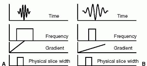FIGURE 3-1 Relationships between time domain, frequency domain, gradients, and slice width are illustrated. In (A), the time domain shows a short radio frequency (RF) pulse, applied to excite a wide frequency range, which in conjunction with a strong gradient produces a slice with the desired physical width. In contrast, in (B), a long RF pulse is applied to excite a narrow frequency range, which in the presence of a weak gradient will excite the same physical slice width as in (A).

Each aspect of slice selection can be controlled by adjusting the slice selection gradient, including orientation, which is realized by changing the gradient direction, and slice thickness, which is adjusted by selecting the BW of the RF pulse in conjunction with appropriate selection of the gradient strength.

SPATIAL ENCODING

A magnetic gradient applied to the body differentiates regions within the slice with respect to their resonance frequency. At one end of the body, the gradient subtracts from the main magnetic field, and at the other end of the body the gradient adds to the main magnetic field. Therefore, the spins ranging from one end of the body to the other resonate at a number of frequencies. These spins generate a signal that contains a continuum of frequencies when the gradient is applied. Although the net signal may look complex, it is simply composed of a sum of sine and cosine waves, each at a discrete and separate frequency (see Fig. 3-2). The FT is a mathematical operation that allows the complex waveform to be analyzed into its component frequencies. The output of the FT routine is the amplitude of each component frequency. By Fourier transforming the signal acquired when a gradient is applied, this allows the amplitude of the individual frequencies to be determined. It can be appreciated that the amplitude of each frequency component when arranged in ascending order corresponds to a projection through the body in a direction perpendicular to the applied gradient.

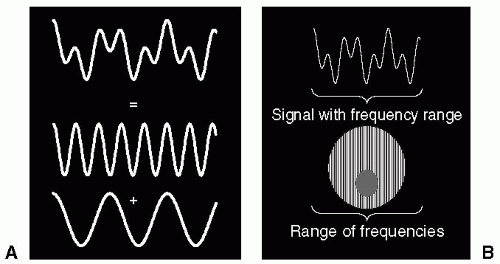FIGURE 3-2 The principal of encoding frequency information is illustrated. In (A) a complex signal waveform is seen, and below it are shown the two primary (pure) frequencies that make up the signal. In this case, the addition of two distinct primary frequencies makes up a relatively complex signal waveform. In (B), a physical object is represented with a gradient applied across it. The gradient imposes a range of (pure) frequencies across the object. The top panel shows the composite signal, which is composed of many distinct frequencies that are emitted by the selected slice of the object.

If the sample were one-dimensional, then a single FT would be sufficient to image it, i.e. to find the amplitude corresponding to each point along the sample. However, most imaging situations are at least 2D, and sometimes 3D. To image a 2D sample, a 2D treatment of the signal must be applied. To see how this is achieved, consider a gradient applied for a period of time as being deconstructed into a series of gradients, each applied for a short time duration, e.g. a single gradient applied for 7 ms is equivalent to seven gradients of equal magnitude applied for 1 ms duration, each applied in a contiguous manner. Therefore, conceptually, it is possible to “split up” the sampling of signal in the presence of a gradient into a series of separately applied gradients, each applied for a short duration. Such an approach is used to encode a 2D image (see Fig. 3-3).

In the 2D signal encoding situation, one dimension is acquired during the application of a single, long duration, gradient (i.e., achieving one dimension of spatial encoding); whereas the second dimension is acquired by application of a series of short duration gradients, each gradient applied orthogonal to the initial spatial encoding gradient, Fig. 3-3. The resulting 2D signal distribution is termed k-space, or phase space. K-space has many properties of interest to MRI and these will be dealt with in greater detail in subsequent chapters. The main point to be made here is that,
conventionally, each line of k-space requires application of two gradients:

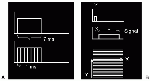FIGURE 3-3 The anatomy of a gradient is illustrated. In (A), the top figure represents a gradient applied for duration 7 ms with a uniform amplitude. In the lower panel, the same gradient is represented as seven separate gradients, each applied for duration 1 ms, and arranged in a contiguous manner. This illustrates that a continuously applied gradient can be split into several subgradients. In (B), two gradients are applied to encode one line of k-space. In this case, a short (phase encoding) gradient is applied before the longer (read-out) gradient. The longer gradient is responsible for reading out the signal associated with one line of k-space, and is applied in the same manner for each line. The shorter gradient is applied in an incremental manner such that it results in reading out successive lines. In effect, multiple applications of a series of short gradients are equivalent to a single long gradient, with each gradient applied in an orthogonal direction.

A short duration gradient, applied to prepare the signal, termed the phase encoding gradient.
A longer duration gradient, applied as the signal is digitally sampled, termed the measurement, or read gradient.

SIGNAL ECHO

To encode data in k-space, the free induction decay (FID) signal must be prepared (i.e., by application of the short duration gradient) before sampling a line of k-space (i.e., using the longer read out gradient). This requires delaying the signal acquisition from the start of the FID, which is generally timed from the middle of the slice selection process. Delaying the signal in MR (magnetic resonance) is achieved by recalling the signal at a later time as an “echo.” By means of an echo, the required signal delay can be achieved and imaging (i.e., spatial encoding of data) can be accomplished. There are three types of echo, as follows:

Each echo has a distinct set of properties that dramatically affect the contrast achieved in MRI.

GRADIENT ECHO

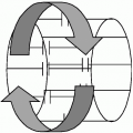
Application of a gradient to the spin system will dephase spins due to the spatial distribution of frequencies imposed by the gradient, that is, because all the spins are precessing at different rates they rapidly lose phase coherence and the signal is observed to decay. At some point later in time, when the spins have reached a certain degree of spin dephasing, the polarity of the gradient is reversed and applied at a constant level (see Fig. 3-4). Under the influence of this reversed gradient, spins at each location experience a reversal of their relative frequencies and they come back into focus. As spins come into phase alignment the signal increases in amplitude; this is the so-called echo signal. When the reverse polarity gradient has been applied for a period of time equal to the initial dephasing gradient the spins are at their highest level of refocusing, corresponding to the echo peak. As the reverse polarity gradient is left on for a further time period, the spins go past their focus condition, and continue to dephase, but in the opposite direction to their initial dephasing pattern. Therefore, application of the reverse gradient results in signal growth (to the echo peak) followed by signal decay. This symmetric rise, peak, and decay of signal constitute the echo signal.

By convention, the “leading” and “trailing” spins are represented diagrammatically with the understanding that, in between these two extremes, there exists a continuum of spin phases, Fig. 3-4. In Fig. 3-4, at the start of the gradient echo process, the leading and trailing spins are represented as precessing clockwise and counterclockwise, respectively, representing the relative precession due to the applied gradient. At the end of the initial gradient application period, the relative phases of the leading and trailing spins are shown in Fig. 3-4, indicating the condition of spin dephasing; complete dephasing is not shown, although in reality, the spins typically undergo many complete revolutions relative to each other. Note that the relative direction of spin precession at the end of the initial gradient period is the same as at the start of the initial gradient period, that is, the leading and trailing spins are represented as precessing clockwise and counterclockwise, respectively. Immediately upon reversal of the gradient polarity, the relative position of the leading and trailing spins remain unchanged, but it is the direction of precession that changes. Owing to this change of direction, the spins gradually come closer together in phase until at the echo peak they reach the point where they are the closest to fully rephrased.
We note that they will never fully rephase, due to the random effects of T2 relaxation. If the second, reverse polarity gradient is continued past the echo peak, the spins continue to dephase relative to each other, and the signal decays accordingly.

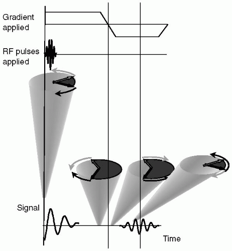FIGURE 3-4 The state of the spin system at key points in the gradient echo procedure is illustrated. At the start of the sequence all spins start off in phase, and in the presence of a gradient, spins precess with a range of frequencies. Relative to the central frequency, some spins appear to precess counter-clockwise, whereas some spins precess clockwise. As the gradient continues to be applied the spins continue to dephase and the signal decreases. At the point where the gradient is reversed, the spins are physically in the same positions as they were immediately before the gradient reversal (i.e., a high degree of dephasing). However, at this point the relative direction of precession is reversed for the representative spins shown. Consequently, as the gradient continues to be applied the phase of the spins gradually comes back into focus (forming the echo peak). Following the echo peak the gradient is still applied and the spins continue to dephase, resulting in echo decay.

A gradient-recalled echo (GRE) “pulse sequence” is shown in Fig. 3-5. The pulse sequence is a diagrammatic representation of the gradients and RF, with strength, polarity and timing shown, that are required to acquire a line (or lines) of k-space. Each line of the pulse sequence represents an individual component: the RF pulse is applied by the scanner, while the echo signal is emitted by the body; the gradients: slice, measurement, and phase are shown; and the digital sampling window, when data are acquired for assembly into k-space, is indicated. Generally, the slice, measurement, and phase encoding gradients are orthogonal to each other. The combination of RF and slice selection gradient achieves the slice selection procedure; the measurement gradient generates the GRE; and the phase encoding gradient, represented as being applied multiple times, is used to encode each line of k-space. Therefore, the basic GRE

Only gold members can continue reading. Log In or Register to continue