K-Space
Mark Doyle
K-space is the “raw data” for magnetic resonance imaging (MRI). The data acquired by the scanner are assembled and arranged internally into individual k-space arrays. Each individual image is derived from a k-space matrix, for example, for one slice imaged at 20 cardiac phases, there are 20 corresponding k-space arrays. In most imaging modalities, the correlation between the physical property sampled and the manner in which data are arranged to form an image is generally intuitively obvious. In MRI, k-space is acquired and an image generated in a manner that is not naturally intuitive. However, k-space is a feature that may have advantages over other modalities:
K-space breaks the one-to-one correspondence between the position of the receiver and the orientation of the image.
It allows arbitrary slice angulation.
It allows reduction in scan time by post-processing of k-space.
It allows parallel imaging to reduce scan time.
It allows image contrast to be altered.
This contrasts with ultrasound:
Image orientation is directly proportional to the position of the probe
Operator dependence
Limited imaging window
And with nuclear medicine:
Orientation of detector array determines image orientation.
Projection reconstruction (PR) produces uneven resolution.
K-SPACE
An appreciation of k-space is central to the understanding of MRI and is explanatory of the origin of its advantages over other modalities. Mathematically, k-space can be succinctly and compactly described by a single equation, which to a mathematician fully explains k-space. However, to a nonmathematician, in general, it is just a series of meaningless symbols. Here we will discuss and explore k-space by means of a series of illustrations, and at the conclusion of this exploration, the equations will be presented. Increased understanding will likely be gained as exposure to the concepts involved occurs.
K-SPACE DIMENSIONS
Physically, k-space is a matrix of data, with dimensions that are typically square, and typically, these are in powers of 2:
128 × 128
256 × 256
512 × 512
The highest concentration of signal is located towards the k-space center. To generate an image, the k-space data are Fourier transformed (see Fig. 24-1). Sometimes, this operation is referred to as a fast Fourier transform (FFT). This is due to a mathematical shortcut that was discovered for matrices with dimensions of powers of 2. The image generated by this mathematical operation has a physical size identical to that of the original k-space matrix:
128 × 128
256 × 256
512 × 512 respectively.
In this respect, there is a one-to-one correspondence between the number of k-space points and the number of image points. Also note that the image features fit within the square (or rectangular) field, termed the field of view (FOV).
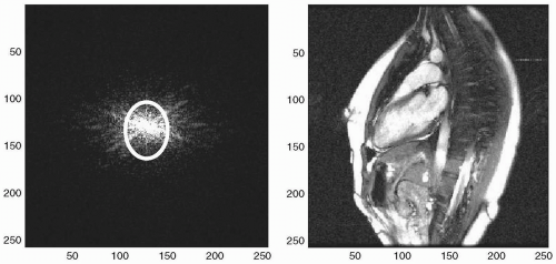 FIGURE 24-1 The k-space matrix represented here is a 2D image of signal intensity. The highest concentration of signal is toward the center of k-space (circled). In this example, k-space has the physical size of 256 × 256 pixels. The corresponding image is generated by performing a Fourier transform on the k-space data. Note that the dimensions of the image are also 256 × 256 pixels. |
PROJECTIONS
Consider an image of a rectangle within a square FOV. The rectangle has a uniform intensity and no internal detail (see Fig. 24-2). Also, there is no noise in this perfect (if somewhat bland) image. In this case the corresponding k-space matrix exhibits a clear pattern of horizontal and vertical symmetry. An alternative way of viewing the k-space data is to represent the signal intensity as a three-dimensional (3D) surface. When viewed in this manner, it is easier to appreciate that along each major axis the signals represent decaying
sinusoidal patterns. One property of k-Space is that any line passing through the center can be Fourier transformed to represent a projection of the object corresponding to the orientation of that line (see Fig. 24-3). In the case of the rectangular image, the FFT of the horizontal central line represents a projection through the rectangular object along the horizontal axis, and the FFT of the vertical line represents a projection through the rectangular object along the vertical axis. Therefore, k-space has the property that symmetry in the object is reflected in symmetry in k-space. Consider the k-space representation of a square object; in this case, k-space demonstrates symmetry along both major axes. Similarly, a circular object results in a k-space pattern that is circularly symmetric, with all lines passing through the center being essentially identical.
sinusoidal patterns. One property of k-Space is that any line passing through the center can be Fourier transformed to represent a projection of the object corresponding to the orientation of that line (see Fig. 24-3). In the case of the rectangular image, the FFT of the horizontal central line represents a projection through the rectangular object along the horizontal axis, and the FFT of the vertical line represents a projection through the rectangular object along the vertical axis. Therefore, k-space has the property that symmetry in the object is reflected in symmetry in k-space. Consider the k-space representation of a square object; in this case, k-space demonstrates symmetry along both major axes. Similarly, a circular object results in a k-space pattern that is circularly symmetric, with all lines passing through the center being essentially identical.
 FIGURE 24-2 An example image of a uniform rectangular object with no internal detail. In this case, the rectangle is 30 pixels wide and 70 pixels long, within a field of view of 128 × 128 pixels. The corresponding k-space representation is shown here as a 3D surface plot, as opposed to the more common intensity plot of Fig. 24-1. Note that in this case, k-space data lies predominantly along the major axes, with data along one axis demonstrating definite oscillations, whereas data along the other axis appears smoother. |
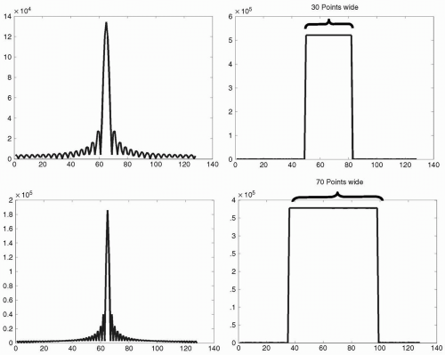 FIGURE 24-3 For the k-space data of Fig. 24-2, the central line of k-space along the axis with dominant oscillations is extracted (top left), and the corresponding 1D Fourier transform data presented as a 1D profile (top right). Here, the profile data has a square appearance, with the plateau of the shape being of width 30 points. This corresponds to the width of the rectangle of the original image in Fig. 24-2. The central line along the perpendicular axis of k-space is represented in the lower panel, and the corresponding 1D Fourier transform profile is shown as a square function of width 70 points (lower right), corresponding to the height of the rectangle of Fig. 24-2. It is apparent that the central lines of k-space correspond to projections through the image, which become apparent when viewing the Fourier transformed data. |
PROJECTION RECONSTRUCTION
In the preceding text, we considered the example of two special lines of k-space
Horizontal
Vertical
However, there are an infinite number of lines that pass through the center of k-space, that is, lines not
confined to the two primary axes. By acquiring these lines, enough data can be acquired to generate an image by back PR. To appreciate the relationship between k-space and the gradients applied to the body, consider applying a horizontal gradient to the selected slice: it results in columns of spins with the same frequency. The signal acquired in the presence of this gradient has that frequency information directly encoded in it. When the signal is Fourier transformed into the frequency domain, the data relates directly to projections of the object. The PR method was used in CT and radionuclide imaging and can also be used in MRI. By acquiring multiple lines through the center of k-space and Fourier transforming the magnetic resonance signal, a sufficient number of projections can be generated to form a PR image. The unique features of lines that pass through the center of k-space are that they can be produced by application of one imaging gradient. As a practical aside, we note that a gradient in any direction can be generated by a combination of three orthogonal gradients, which, if applied simultaneously in different strengths, effectively combine to form a single gradient applied at some intermediate orientation. When viewed in terms of k-space, the PR data can be represented as a series of lines, each passing through the center of k-space. In this representation, it is apparent that the highest density of points in the PR data set is toward the center whereas the lines are sparser toward the periphery. PR images have several artifacts, as follows
confined to the two primary axes. By acquiring these lines, enough data can be acquired to generate an image by back PR. To appreciate the relationship between k-space and the gradients applied to the body, consider applying a horizontal gradient to the selected slice: it results in columns of spins with the same frequency. The signal acquired in the presence of this gradient has that frequency information directly encoded in it. When the signal is Fourier transformed into the frequency domain, the data relates directly to projections of the object. The PR method was used in CT and radionuclide imaging and can also be used in MRI. By acquiring multiple lines through the center of k-space and Fourier transforming the magnetic resonance signal, a sufficient number of projections can be generated to form a PR image. The unique features of lines that pass through the center of k-space are that they can be produced by application of one imaging gradient. As a practical aside, we note that a gradient in any direction can be generated by a combination of three orthogonal gradients, which, if applied simultaneously in different strengths, effectively combine to form a single gradient applied at some intermediate orientation. When viewed in terms of k-space, the PR data can be represented as a series of lines, each passing through the center of k-space. In this representation, it is apparent that the highest density of points in the PR data set is toward the center whereas the lines are sparser toward the periphery. PR images have several artifacts, as follows
Uneven resolution
○ Higher at center
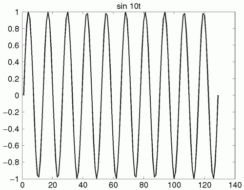
FIGURE 24-4 Because each point of k-space is digitally sampled, the properties of digital sampling are considered. Here a 1D sinusoidal oscillating time varying waveform is sampled at regular intervals for a total time Ttotal. The digital sampling process is fully described by the sampling rate and the sampling duration.
○ Lower at periphery
Star artifact from bright objects
SIGNAL INFORMATION
The time domain signal obtained in MRI is digitally sampled (see Fig. 24-4). The digital sampling process is characterized by two variables:
Sampling duration
When sampling data that relates to frequency information, a natural means of assessing the appropriateness of the measuring parameters is to consider the bandwidth (BW) of the measured signal (see Fig. 24-5). The BW of the measured signal is determined by the formula:
1/Tsample
Where Tsample is the sampling interval time between individual points. Under conditions that the BW matches or exceeds the highest frequency component in the signal, the signal is correctly represented. Another parameter to consider is the frequency per point of
the frequency domain signal (see Fig. 24-6). This is determined by the total sample interval (Ttotal):
the frequency domain signal (see Fig. 24-6). This is determined by the total sample interval (Ttotal):
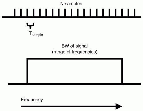 FIGURE 24-5
Get Clinical Tree app for offline access
Related posts:Stay updated, free articles. Join our Telegram channel
Full access? Get Clinical Tree


|