Gradient Echo
Mark Doyle
OVERVIEW
Gradient echo imaging is one of the fundamental imaging sequences used in cardiovascular applications. This is mainly because it lends itself easily to cine imaging, and is therefore used in applications that assess cardiovascular function, such as the following:
Velocity
Perfusion
Delayed enhancement viability imaging
These application areas may either directly use classical gradient echo imaging or some variant on the basic sequence. Important variants on gradient echo imaging and specialized applications are discussed in more detail in separate chapters. Here, the basics of the technique are introduced, together with a brief outline of how gradient echo imaging is applied to assess myocardial function, blood flow, and perfusion.
GRADIENT ECHO IMAGING—BASIC PRINCIPLES
Spatial information is encoded by application of magnetic gradients to the spin system. The local magnetic field experienced by each spin, B0, results in the spin precessing at a fixed angular frequency, ω, which is characteristic of the gyromagnetic ratio, γ, of the nuclear species. The relationship linking these three qualities is termed the Lamor equation:
Therefore, if the local magnetic field varies in a linear manner, from a low field at one position in the body to a high field at another position (a magnetic gradient), the nuclear spins will experience a linear range of frequencies. Therefore, signal acquired in a magnetic gradient directly relates spin frequency to spatial position in the one-dimensional (1D) case. However, the body is 3D. After performing slice selection, the problem of imaging reduces to a 2D situation. However, this may present a conceptual problem, that is, if a linear gradient relates only to one dimension, then how is the second dimension encoded? To address this, we quickly introduce the conceptual framework of k-space: which can be regarded as a signal space in which frequency information is encoded along the two dimensions. Other chapters give a fuller description of k-space, but here the important features to be aware of are that the 2D gradient echo signals are arranged to fill k-space directly. Once the k-space data set has been compiled, application of a single Fourier transform operation is sufficient to generate an image. Therefore, k-space forms the signal domain and the Fourier transform, which is a signal processing operation, is applied to form an image. In 2D magnetic resonance imaging (MRI), the k-space signal is arranged in a 2D matrix and is commonly represented as a series of parallel lines. Most MRI sequences populate k-space one line at a time. To encode each k-space line requires application of two separate gradients:
Frequency encoding gradient, for example, X
Phase encoding gradient, for example, Y
Note in Fig. 17-1, illustrating the acquisition of two lines of k-space, that the frequency encoding gradient is applied identically for each line. However, the phase encoding gradient is required to ensure that successive lines are stepped through to cover the second dimension of k-space. Also note that the phase encoding gradient is applied before signal detection, which occurs at the frequency encoding stage.
SIGNAL PREPARATION
The phase encoding gradient is applied before the signal read out because the spin system has to be prepared.
Therefore, we require the signal to be delayed from its inception at slice selection to the time of detection. This small delay is accomplished by the maneuver of forming a signal echo. Here, we will consider the gradient echo variant of forming a signal echo.
Therefore, we require the signal to be delayed from its inception at slice selection to the time of detection. This small delay is accomplished by the maneuver of forming a signal echo. Here, we will consider the gradient echo variant of forming a signal echo.
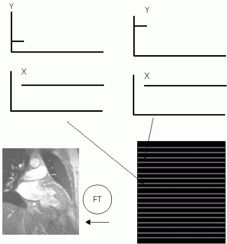 FIGURE 17-1 K-space encoding is illustrated. Each line of the k-space matrix (series of lines) are encoded by applying an X gradient in a uniform manner as indicated. Each line of k-space is distinguished from other lines by the Y gradient applied. The Y gradient is applied in the stepped manner indicated in the top panel. Therefore, to acquire the complete k-space matrix requires successive application of the sequence: the Y gradient applied in a stepped manner, and the X gradient applied in a uniform manner. When the k-space matrix is complete, application of the image-processing step of the Fourier transformation (FT) is all that is required to form an image. Note that there is a time delay between application of the X and Y gradients. |
GRADIENT ECHO
By applying a positive gradient for a time period, and following it by a negative gradient, we can appreciate that the spins initially advance in phase in the positive gradient and reverse in phase in the negative gradient (see Fig. 17-2). Since spins at physically different locations along the gradient direction experience a range of rotation frequencies, when the positive gradient is applied, the signal is observed to decay as spins progressively lose phase coherence with respect to each other. Conversely, application of the negative gradient results in signal regrowth, as spins progressively come back into phase, forming an echo peak. Because the negative gradient continues to be applied following the echo peak, the spins progressively lose phase, and signal decay is again observed. Therefore, the positive gradient followed by a negative gradient results in a signal echo, characterized by a signal buildup to a peak, which then decays to zero in a time-symmetric manner. The echo time (TE) is defined as the time from signal origination at slice selection to the echo peak.
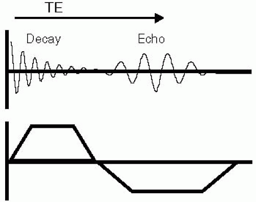 FIGURE 17-2 The time delay between application of the phase encoding and frequency encoding gradients is accomplished by generation of a gradient echo. First, a positive gradient is applied, which causes the signal to decay rapidly, because spins at multiple spatial locations become dephased with respect to each other. This gradient is followed by a negative gradient that refocuses spins. When the spins come into phase, they form an echo peak. After the echo peak is attained, the signal dephases, and again decays. The echo formed by this means is symmetric. The time from spin excitation to the echo peak is termed the echo time (TE). |
GRADIENT-RECALLED ECHO PULSE SEQUENCE
The gradient-recalled echo (GRE) sequence is composed of the following steps:
Phase encoding gradient
Gradient echo formation, which also forms the frequency encoding or measurement gradient
We note that each application of the phase gradient only generates data for one k-space line, and consequently, multiple applications of the basic imaging sequence are required to compile a complete k-space matrix (see Fig. 17-3). Further, to form a cardiac cine image series, multiple k-space matrices are required, that is, one complete matrix for each point in the cardiac
cycle where an image is needed (see Fig. 17-4). Because each k-space matrix is compiled one line at a time, data must be acquired over multiple cardiac cycles to build up the set of k-space matrices required to generate temporally resolved images. This is achieved by synchronizing the acquisition with the cardiac cycle to form a cine image series.
cycle where an image is needed (see Fig. 17-4). Because each k-space matrix is compiled one line at a time, data must be acquired over multiple cardiac cycles to build up the set of k-space matrices required to generate temporally resolved images. This is achieved by synchronizing the acquisition with the cardiac cycle to form a cine image series.
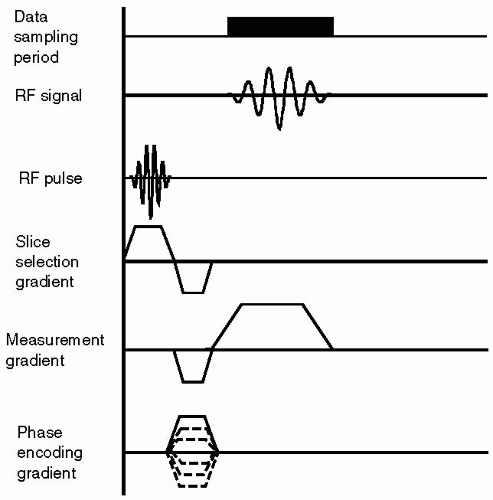 FIGURE 17-3 The gradient echo pulse sequence is shown. Each line represents an activity, such as application of a gradient, an RF pulse, or performing signal detection. The first RF pulse is applied by the system in conjunction with the slice selection gradient, and is the combination that is responsible for accomplishing slice selection. The gradient echo forms the frequency encoding gradient, and data is sampled as the echo is formed. The phase encoding gradient is applied in successive steps as indicated. RF, radio frequency. |
GRADIENT ECHO TERMINOLOGY
Some of the terminology associated with gradient echo imaging is as follows:
TE; echo time
TR; repetition time of the basic “pulse sequence”
Pulse sequence; the imaging procedure, gradient-recalled echo
Typical values for gradient echo imaging parameters are as follows:
TR; low, 4 to 10 milliseconds
TE; short, 1 to 6 milliseconds
Blood signal; bright, owing to flow refreshment
Fat signal; bright, owing to short T1
Myocardium signal; intermediate intensity
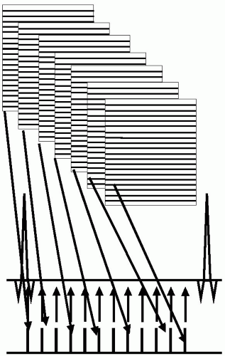 FIGURE 17-4 To acquire a series of images over the cardiac cycle, a series of k-space matrices are required, each matrix corresponding to a point in the cardiac cycle. Multiple cardiac cycles are required to acquire the time-resolved cardiac image series. |
FREQUENCY AND PHASE ENCODING GRADIENTS
To encode each k-space line requires application of the following two separate gradients:
Frequency encoding
Phase encoding
Related posts:
Stay updated, free articles. Join our Telegram channel

Full access? Get Clinical Tree


