Keys to Robust Arterial Spin Labeling in the Clinical and Research Environment
David C. Alsop
Jeroen Hendrikse
Arterial spin labeling (ASL) promises nearly everything that could be desired from a blood flow imaging method: a quantitative measure of blood flow that requires no contrast or radiation and can provide high temporal resolution and suppression of vascular signal. The method is even performed with a magnetic resonance imaging (MRI) scanner where other measures of anatomy and function can be obtained with excellent spatial registration. So why has ASL taken so long to reach clinical use and why is it still far from reaching widespread adoption? The dominant obstacle has been robustness. For use as a clinical (and even clinical research) tool, an imaging technique must provide reliable measures in a broad clinical population within a reasonable period of time. The focus of this chapter is on the factors that can contribute to poor results in ASL studies and methods to minimize their effects.
Signal-to-Noise Ratio
Perhaps the most common yet most avoidable cause of poor results with ASL is a low signal-to-noise ratio (SNR). It is important to remember that the flow-related signal in an ASL acquisition is much lower than in a typical, T1– or T2-weighted image. Because ASL creates competition between flow of labeled blood into the tissue and decay of tracer with T1 relaxation after it arrives, the fractional signal change in an image is of the order of flow times T1. Here, flow must be expressed in units of milliliters per milliliter per second. For example, a conventional average brain blood flow of 50 mL/100 g/min corresponds to 0.008 seconds−1 (where a density of 1.05 g/mL was used).1 For a T1 relaxation time of 1.4 seconds, corresponding to gray matter at 3T, the signal change is thus 1.1%. There are a number of significant additional factors that influence signal change, such as inversion efficiency, noise propagation with subtraction, and especially T1 decay of the label before it arrives in the tissue, but a signal change from ASL of roughly 1% serves as a useful approximation for consideration of SNR.
A common mistake in prescribing ASL pulse sequences is to draw upon experience from T2– or T1-weighted imaging. For example, a high-quality volumetric image of the brain with an excellent gray to white matter contrast-to-noise ratio of 10 can be achieved within 5 to 10 minutes with scan times at a spatial resolution of 1 × 1 × 1 mm2. This usually employs matrix sizes of approximately 256 pixels. What will happen if a scan prescription of this resolution is used for ASL? A noisy image will be produced with absolutely no detectable perfusion signal. Why? An SNR of 20 becomes 0.2 when multiplied by the ASL signal change of 1%. Does this mean that ASL is hopeless because of low SNR? No, it means that we must temper our expectations of spatial resolution to achieve a reliable measure.
Reducing the spatial resolution of an MRI has a dramatic impact on the SNR (Fig. 21.1). Everything else being equal, especially averaging time, the SNR increases as the voxel volume3 increases. So switching from 1 × 1 × 1 mm to 4 × 4 × 4 mm increases SNR by a factor of 64 (i.e., 43). With this reduction of resolution, the ASL SNR of 0.2 reaches 12.8, a fairly respectable value. Those most familiar with anatomic imaging might be dissatisfied with such resolution, but in functional imaging, whether functional MRI, single-photon emission computed tomography, or positron emission tomography, 4-mm resolution is quite respectable. Can one extract the 4-mm resolution image from the 1-mm resolution image by smoothing or other processing? Only partially. Theoretically, smoothing averages the signal but only partially reduces noise. The SNR improvement with smoothing is just the square root of the voxel volume increase. For example, smoothing the 1 × 1 × 1 mm image with a 4 × 4 × 4 mm box kernel will improve SNR only eightfold, compared with the 64-fold improvement when the image is acquired at the lower resolution. This reduced improvement reflects wasted time spent acquiring high-resolution information that is discarded by the smoothing process.
Other, more subtle effects also can contribute to reduced image quality at low SNR. For example, reconstruction of magnitude images can lead to reduced visibility of ASL perfusion differences at low SNR.4,5 Magnitude reconstruction is fairly optimal at high SNR but becomes less optimal as the SNR approaches one. Remember that the MRI has two components that can be thought of as the real and imaginary components of a complex number. Signal appears with a certain ratio of real to imaginary, often referred to as a signal phase. Noise appears independently at both phases. Magnitude reconstruction eliminates uncertainty about the signal phase, but also contributes noise from the phase perpendicular to the signal phase. Noise appears higher and also with a
positive average value on a magnitude image (Fig. 21.1). This bouncing off the noise floor, which leads to nonzero mean values at very low signal values, is due to the Rice-Nakagami noise distribution of MR magnitude data (see Chapter 12). This effect is even more pronounced in multi-coil acquisitions where the coils are combined by a square root of the sum-of-square algorithm. If ASL is acquired without background suppression, typically the label and control image are reconstructed separately (and the signal level is high), this noise rectification issue is avoided. However, when complex subtraction is used (and residual differential signal is low) or when background suppression is employed (where signal is low to begin with), the use of alternate phasing and coil combination strategies is preferable.4
positive average value on a magnitude image (Fig. 21.1). This bouncing off the noise floor, which leads to nonzero mean values at very low signal values, is due to the Rice-Nakagami noise distribution of MR magnitude data (see Chapter 12). This effect is even more pronounced in multi-coil acquisitions where the coils are combined by a square root of the sum-of-square algorithm. If ASL is acquired without background suppression, typically the label and control image are reconstructed separately (and the signal level is high), this noise rectification issue is avoided. However, when complex subtraction is used (and residual differential signal is low) or when background suppression is employed (where signal is low to begin with), the use of alternate phasing and coil combination strategies is preferable.4
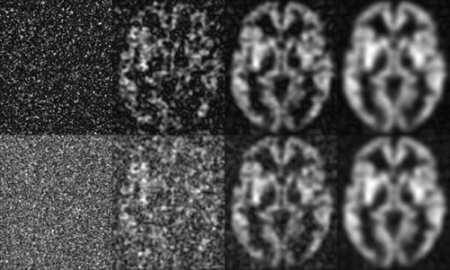 FIGURE 21.1. The effect of resolution on the signal-to-noise ratio (SNR) of arterial spin labeling (ASL). Random noise was added to data acquired at 3 mm in plane resolution to simulate the effect of a change in voxel size on SNR. Left to right: Images with a cubic resolution of 1 mm, 2 mm, 3 mm, and 4 mm are shown. The upper row uses a phased reconstruction to reduce magnitude noise and offset, and the bottom row used magnitude reconstruction. |
There are a number of strategies to increase SNR beyond simply reducing resolution. None are as powerful, however. Suppose a technique increases SNR by a factor of three, for example. The corresponding increase in SNR would allow us to reduce the voxel size in each direction by a factor of cube root of 3 or only 30%. One of the weakest approaches to SNR improvement is signal averaging because SNR only improves as the square root of time3. To gain a threefold improvement in SNR requires lengthening the scan time by a factor of 9 (i.e., 36 minutes instead of 4 minutes). This is not only an unreasonable increase in scan time, it also increases the likelihood of motion artifacts substantially. Signal averaging is more desirable when orders of magnitude of improvement in imaging time are possible. For example, averaging an 8-second single-shot acquisition over 4 minutes (or 30 averages) improves the SNR by a factor of 5.5.
One factor that should definitely be optimized for an ASL acquisition is the sensitivity of the coils used for signal reception. The use of dedicated coil arrays for the head, instead of a single-channel (birdcage) receiver head coil, has had a major impact on sensitivity. Although it has been argued that multicoil arrays for the head produce limited SNR improvement toward the center relative to an optimized single coil, most general purpose birdcages that receive coils for the head are designed to provide coverage of the entire head and neck, not just the brain. This larger coil sensitivity volume (i.e., the region from where the coil picks up signal) adds (body-generated) noise emanating from the neck and shoulders that degrades SNR of the head.6 Even many clinical head array coils may not be optimal for the center of the head. That said, fantastic improvements in SNR, very close to the surface of the brain, can be achieved with high-density (e.g., 64 up to 128 elements) array coils. High-density arrays also improve the SNR of parallel imaging acceleration, a technique that might be desirable to increase speed and even freeze motion with single-shot acquisition.7 Here, the spatially more distinct coil sensitivity profiles of the individual coil elements of high-density arrays allow higher acceleration at very low parallel imaging-related noise enhancement. One danger of high-density arrays is that high signal from the scalp and edge of the brain could produce artifacts from motion and other sources that could propagate into the lower SNR brain center because motion causes ghosts across the image in the phase direction. Background suppression and careful coil combination algorithms may be necessary to achieve the full advantages of high-density coil arrays.
Another hardware approach to improving SNR is acquiring images at higher field strength. For any type of imaging, the SNR gain with field strength reflects a competition between the roughly linear increase in SNR per unit time, a potential loss of imaging efficiency because of susceptibility or power deposition restrictions, and the potential change in signal or contrast for the particular imaging technique. For example, the improved SNR of
T1-weighted imaging at higher field strength appears to be partially offset by the reduced T1-contrast between tissues.8 ASL contrast increases substantially with field strength because the T1 relaxation time of both blood and tissue increases. ASL depends exponentially on T1 relaxation time of blood because of delayed arrival of the label in the tissue of interest. Accumulation of signal in tissue also increases as T1 relaxation time increases. Most analyses show a major improvement of SNR from moving to 3 or 4T from 1.5T (Fig. 21.2).9 Employing 7T or higher magnetic field strength is still an area of development. Increases in T1 relaxation times are clear, but challenges of radiofrequency (RF) and B0 field inhomogeneity contribute to reduced overall sensitivity and potentially labeling inefficiency.10,11 Despite the advantages of high field strength, it is important to remember that excellent quality ASL can be performed at the more widely available 1.5T with much less hassle with regards to B0 and RF inhomogeneity and specific absorption rate concerns.
T1-weighted imaging at higher field strength appears to be partially offset by the reduced T1-contrast between tissues.8 ASL contrast increases substantially with field strength because the T1 relaxation time of both blood and tissue increases. ASL depends exponentially on T1 relaxation time of blood because of delayed arrival of the label in the tissue of interest. Accumulation of signal in tissue also increases as T1 relaxation time increases. Most analyses show a major improvement of SNR from moving to 3 or 4T from 1.5T (Fig. 21.2).9 Employing 7T or higher magnetic field strength is still an area of development. Increases in T1 relaxation times are clear, but challenges of radiofrequency (RF) and B0 field inhomogeneity contribute to reduced overall sensitivity and potentially labeling inefficiency.10,11 Despite the advantages of high field strength, it is important to remember that excellent quality ASL can be performed at the more widely available 1.5T with much less hassle with regards to B0 and RF inhomogeneity and specific absorption rate concerns.
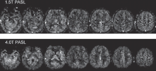 FIGURE 21.2. Comparison of pulsed arterial spin labeling acquired at 1.5T (top) and 4T (bottom). Signal-to-noise ratio is improved with the higher field acquisition. (Adapted from ref. 9.) |
A final factor in determining SNR is the efficiency of acquisition. Sequences with long readout trains that refocus the signal and encode or average it are generally most SNR efficient for imaging with ASL preparation. In other words, one should avoid spending a lot of time on the spin-label part (e.g., background suppression, labeling, etc.) and then just reading out a small amount of the information needed to form ASL images. Rapid acquisition with relaxation enhancement (RARE)12,13 (turbo-spin echo, fast-spin echo) and related hybrid techniques, such as gradient and spin echo14 and stack of spirals RARE15,16 or balanced steady state free precession17 (true fast imaging with steady state precession), are some of the most efficient sequences. Long readout train echo-planar or spiral acquisitions have theoretically slightly lower efficiency but perform well in practice, although efforts to reduce artifacts with parallel imaging18 can further degrade SNR efficiency. Unrefocused acquisitions, such as low flip angle gradient echo with spoiling (e.g., spoiled-gradient echo, fast low angle shot, T1 fast-field echo) typically have greatly reduced efficiency and are less desirable.
Strategies to Minimize Motion Sensitivity
In brain tissue, the volume of blood that flows through the microvasculature in a few seconds is just a small percentage of the entire voxel volume. For this reason, the observed ASL signal change from ASL will be minute (i.e., typically <1% of the total signal from tissue). Thus, ASL perfusion images can be overwhelmed by fluctuations between images caused by motion. Even snapshot imaging techniques cannot eliminate this motion because the interval between label and control images is always more than 1 second. Even the tiniest misregistration between label and control image will cause the difference in images to be dominated by the difference in tissue signal and will swamp the perfusion signal. Robust imaging with ASL requires a solution to this problem.
The simplest strategy to avoid motion artifacts is to acquire the label and control images as close in time as possible to each other. This reduces the time available for a shift in position. Even if image acquisition and averaging continue for many minutes, alternating between label and control acquisition can be used to keep the label and control images within one repetition time, typically just a few seconds, of each other. More detail on label and control alternation and its interaction with k-space acquisition is provided in the image acquisition section. This alternation strategy is almost always used and is quite successful, but residual motion artifacts and noise are usually still present when used alone.
Two general strategies have been used to further minimize motion effects in ASL. The first is to detect motion and realign the images to correct for the motion. This realignment is typically performed as a postprocessing step, where automated algorithms can detect and correct motion from a series of images. In principle, realignment can also be performed during the acquisition using low-resolution images, sometimes called navigators, to detect the motion and adapt to it.
The second motion artifact reduction strategy is to suppress the background signal intensity with one or more inversion pulses. Background suppression, discussed more fully in other chapters, can reduce the signal from the image by up to 100 times while largely preserving the ASL signal change. Background suppression methods have reduced ASL sensitivity to motion artifacts by reducing the severity of subtraction artifacts when patient motion occurs during a label and control pair.15,19 Still, because ASL relies on the averaging of a series of pairs of label and control images, repeated patient motion during the minutes of ASL data acquisition will result in deterioration of the ASL images. Background suppression and navigator strategies can in principle be combined to provide the greatest robustness to motion.
Acquisition Methods for Robust Arterial Spin Labeling
Related posts:
Stay updated, free articles. Join our Telegram channel

Full access? Get Clinical Tree


