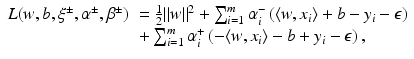
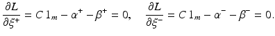
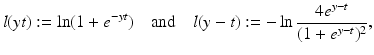
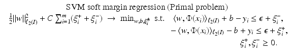
,  , where for simplicity only
  is considered, and
  . The aim of the following sections is to learn a target function
  from given training samples
  . A distinction is made between classification and regression tasks. In classification
  is a discrete set, in general as large as the number of classes the samples belong to. Here binary classification with just two labels in
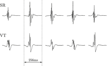
  was most extensively studied. An example where binary classification is useful is SPAM detection. Another example in medical diagnostics is given in Fig. 1. Here it should be mentioned that in many practical applications, the original input variables are pre-processed to transform them into a new useful space which is often easier to handle but preserves the necessary discriminatory information. This process is also known as feature extraction .
 is not countable here. The above examples, as all problems considered in this paper, are from the area of supervised learning. This means that all input vectors come along with their corresponding target function values (labeled data). In contrast, semi-supervised learning makes use of labeled and unlabeled Data, and in unsupervised learning labeled data are not available, so that one can only exploit the input vectors x i . The latter methods can be applied for example to discover groups of similar exemplars within the data (clustering), to determine the distribution of the data within the input space (density estimation), or to perform projections of data from high-dimensional spaces to lower-dimensional spaces. There are also learning models which involve more complex interactions between the learner and the environment. An example is reinforcement learning which is concerned with the problem of finding suitable actions in a given situation in order to maximize the reward. In contrast to supervised learning, reinforcement learning does not start from given optimal (labeled) outputs but must instead find them by a process of trial and error. For reinforcement learning, the reader may consult the book of Sutton and Barto [97].
2 Historical Background
 and corresponding
  ,
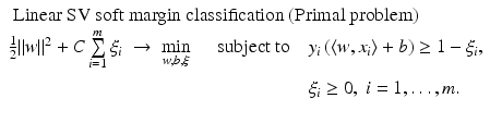
,  a hyperplane
  having minimal least squares distance from the points (x i , y i ):
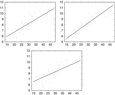
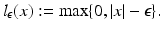
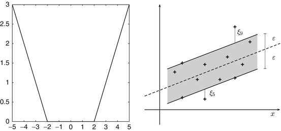
 as in section “Linear Least Squares Classification and Regression” were examined under the name ridge regression by Hoerl and Kennard [49]. This method can be considered as a special case of the regularization theory for ill-posed problems developed by Tikhonov and Arsenin [102]. Others than the least squares loss function like the ε–insensitive loss were brought into play by Vapnik [105]. This loss function enforces a sparse representation of the weights in terms of so-called support vectors which are (small) subsets of the training samples {x i : i = 1, …, m}.
 and γ is the smallest distance between a training point and the hyperplane. For linearly separable points, there exist various hyperplanes separating them.
3 Mathematical Modeling and Applications
Linear Learning
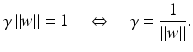
 . In the context of learning, w is called weight vector and b offset, intercept or bias.
Linear Support Vector Classification
 , one can use
 , and the distance of a point
  to the hyperplane is given by
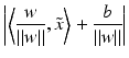
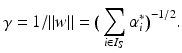
 is the distance of the hyperplane from the origin.
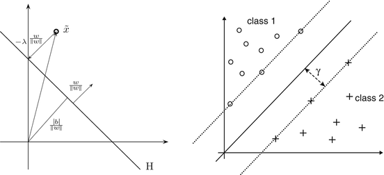
 and distance
  from the origin. The distance of the point
  from the hyperplane is the value
  fulfilling
 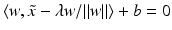 , i.e.,
 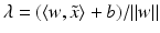 . Right: Linearly separable training set together with a separating hyperplane and the corresponding margin γ
  and
and  . The training set is said to be separable by the hyperplane H(w, b) if
 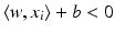 for i ∈ I −, i.e.,
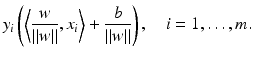
 . The same hyperplane can be obtained as follows: by (3), it holds
 becomes minimal, and the scaling means that
 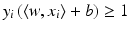 for all
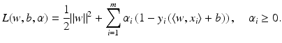
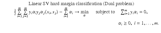
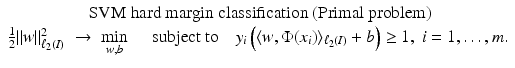
  . Therefore, the hard margin classifier aims to find parameters
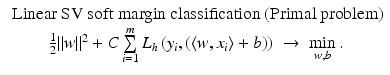
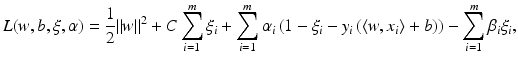
  and b solving the following quadratic optimization problem with linear constraints:
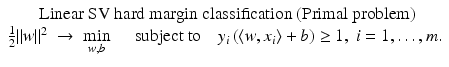

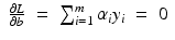
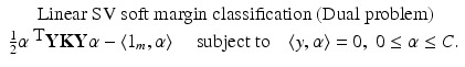
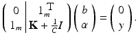
 . Let 1 m denote the vector with m coefficients 1,
  ,
,  ,
, 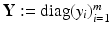 and
and
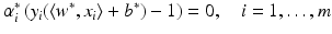
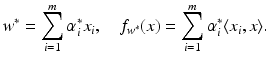
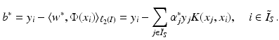
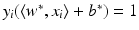 . These are exactly the (few) points having margin distance γ from the hyperplane H(w ∗, b ∗). Define
 have a sparse representation in terms of the support vectors
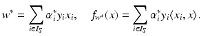
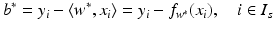
 , where w ∗ is the solution of the above problem. If the slack variable fulfills 0 ≤ ξ i ∗ < 1, then x i is correctly classified, and in the case
 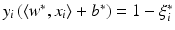 the distance of x i from the hyperplane is
  . If 1 < ξ i ∗, then one has a misclassification. By penalizing the sum of the slack variables, one tries to keep them small.
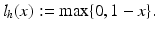
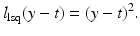
 is called margin based if there exists a representing function l: ℝ → [0, ∞) such that
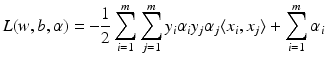
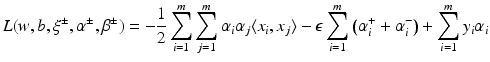
 are again given by (9) and depend only on the few support vectors defined by (8). By the Kuhn-Tucker conditions, the equations
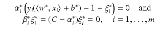
 , i.e., the points x i have margin distance
  from H(w ∗, b ∗). Moreover,
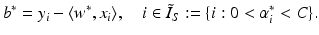
 , i.e., x i has distance
  from the optimal hyperplane.
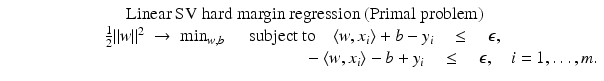
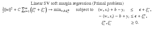
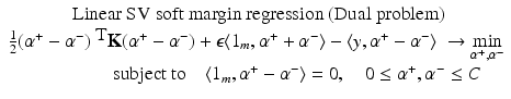
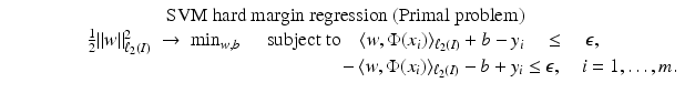
 Linear Support Vector Regression


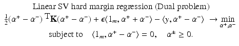
 be the solution of this problem and
  . Then, by (12), the optimal weight and the optimal function have in general a sparse representation in terms of the support vectors x i , i ∈ I S , namely,
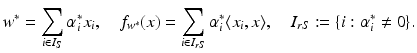

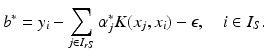
 and consequently, either
  or
or  . Thus, one can obtain the intercept by
 is called distance based if there exists a representing function
  such that
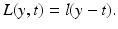
 are the solution of this problem and
 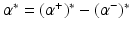 , then the optimal weight w ∗ and the optimal function
  are given by (14). The corresponding Kuhn-Tucker conditions are
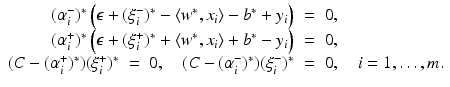

 or
or  . In case
  , this results in the intercept
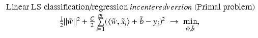
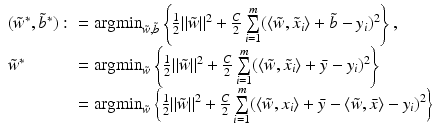
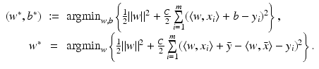
Linear Least Squares Classification and Regression
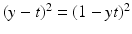 for y ∈ {−1, 1}, the least squares loss is also margin based, and one can handle least squares classification and regression using just the same model with y ∈ {−1, 1} for classification and y ∈ ℝ for regression. In the unconstrained form, one has to minimize
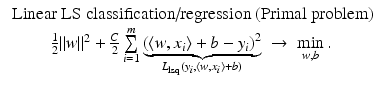
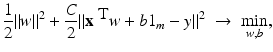
 and
and  . Hence b and w can be obtained by solving the linear system of equations
 , i = 1, …, m. The advantage is that
  , where 0 m is the vector consisting of m zeros. Thus, (19) with
  instead of x i becomes a separable system, and one obtains immediately that
  and that
  follows by solving the linear system with positive definite, symmetric coefficient matrix
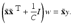
 is just the solution of the centered primal problem without intercept. Finally, one can check by the following argument that indeed
  :
:
 but this is not the coefficient matrix in (19). When turning to nonlinear methods in section “Nonlinear Learning,” it will be essential to work with K = X T X instead of XX T. This can be achieved by switching to the dual setting. In the following, this dual approach is shown although it makes often not sense for the linear setting since the size of the matrix K is in general larger than those of
  . First, one reformulates the primal problem into a constrained one:
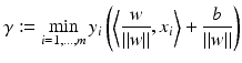
Nonlinear Learning
 into a feature space
  , where I is a countable (possibly finite) index set, by a nonlinear feature map
 becomes linear in the feature space
  .
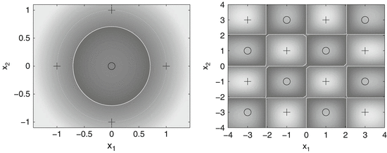
. is linearly separable. In practical applications, in contrast to this example, the feature map often maps into a higher dimensional, possibly also infinite dimensional space.
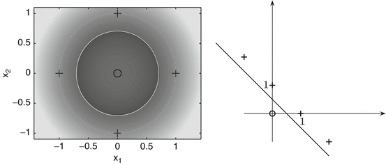
 (left) and become separable in the feature space
  , where
  (right)
 , this approach results in the successful support vector machine (SVM).
Kernel Trick
 , define a kernel
  associated with
  by
by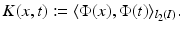
 explicitly.
 forms an orthonormal basis of a reproducing kernel Hilbert space (RKHS)
  . These spaces are considered in more detail in section “Reproducing Kernel Hilbert Spaces.” Then the feature map is defined by
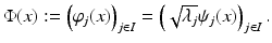
 there exists a unique sequence
  such that
 by (24). Moreover, Parseval’s equality says that
 instead of
  . Using (22) instead of (2) and
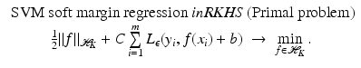
 in (7), the linear models from section “Linear Learning” can be rewritten as in the following subsections. Note again that K is positive semi-definite.
 Support Vector Classification
 is associated with a Mercer kernel K, then
  lies in the RKHS
  , and the model can be rewritten using (25) from the point of view of RKHS as
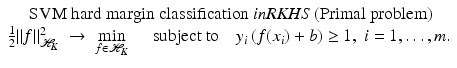
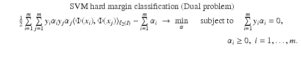
 become
 knowing only the kernel and not the feature map itself. One property of a Mercer kernel used for learning purposes should be that it can be simply evaluated at points from
  . This is, for example, the case for the Gaussian. Finally, using (10) in the feature space, the intercept can be computed by
 by using
  .
. 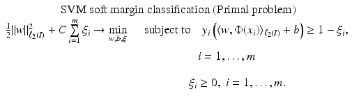
 is associated with a Mercer kernel K, the corresponding unconstrained version reads in the RKHS
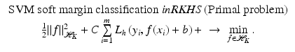

Support Vector Regression
 is associated with a Mercer kernel K, then
 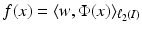 lies in the RKHS
  , and the model can be rewritten using (25) from the point of view of RKHS as
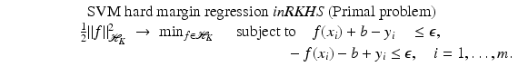
 defined by (26). Let
  be the solution of this dual problem and
  . Then one can compute the optimal function
  using (14) with the corresponding feature space modification as
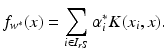
 :
:
 , one can compute the optimal function
  as in (28) and the optimal intercept using (17) as
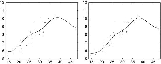
Relations to Sparse Approximation in RKHSs, Interpolation by Radial Basis Functions, and Kriging
 be a RKHS with kernel K. Consider the problem of finding for an unknown function
  with given
  , i = 1, …, m an approximating function of the form
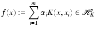
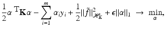
 -norm of the error and to penalize the so-called ℓ 0-norm of α given by
 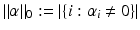 to enforce sparsity. Unfortunately, the complexity when solving such ℓ 0-penalized problems increases exponentially with m. One remedy is to replace the ℓ 0-norm by the ℓ 1-norm, i.e., to deal with
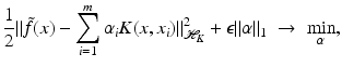
 is defined by (26). With the splitting
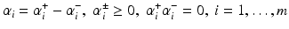
 , the sparse approximation model (30) has finally the form of the dual problem of the SVM hard margin regression without intercept:
Related posts:
 Segmentation with Shape Priors: Explicit Versus Implicit Representations
 Set Methods for Structural Inversion and Image Reconstruction
Stay updated, free articles. Join our Telegram channel

Full access? Get Clinical Tree


