Left Ventricular Systolic Performance and Pathology
OF ALL THE INDICATIONS FOR echocardiography, the evaluation of left ventricular (LV) systolic function is perhaps the most common; in part because it is not only the best understood parameter of cardiac function but also because it has consistently been shown to be a predictor of morbidity and mortality. Left ventricular systolic performance is usually assessed in practically every echocardiogram, even if it is not the primary focus of the examination. The American Society of Echocardiography (ASE) recommends that every complete echocardiographic examination should include the evaluation of LV chamber size and function and emphasizes the importance of these measurements for clinical decision making (1).
WHAT IS LEFT VENTRICULAR SYSTOLIC FUNCTION?
LV systolic function describes the contractility of the LV. Contractility of the myocardial fibers of the heart is described by the Frank–Starling relationship whereby increases in preload (left ventricular end diastolic pressure [LVEDP]) result in increased contractility. Therefore, contractility or systolic function is load dependent and strictly speaking, should be assessed over a range of preload and afterload. This is not usually clinically feasible and true load-independent assessments of LV systolic function are difficult using echocardiography. Consequently, the preload status at the time of the examination is frequently reported along with the systolic function as the LV chamber dimension either as a diameter, area, or volume. LV thickness or mass is also usually reported with systolic function and LV chamber size to complement the overall estimate of LV systolic performance.
Quantitative Measures of Left Ventricular Systolic Performance
LV systolic performance may be assessed qualitatively or quantitatively with echocardiography. There are a number of parameters which describe LV systolic function, the most commonly used being ejection fraction. Ejection fraction is expressed mathematically as a fraction of a diastolic dimension minus the corresponding systolic dimension divided by the original diastolic dimension, where this dimension can be a linear measurement, an area, or a volume. For example:

where LVEDV is LV end diastolic volume and LVESV is LV end systolic volume. A normal ejection fraction is equal to or greater than 55% for both men and women.
An echocardiographer may become quite efficient and accurate at visually estimating left ventricular ejection fraction (LVEF). However, accuracy and reproducibility are dependent upon the individual interpreter’s skill and interobserver measurements may vary considerably. Consequently, calibrated measurements are preferred, and the ASE recommends that even experienced echocardiographers regularly cross-check qualitative evaluations against calibrated measurements (1).
Quantitative Evaluation of Left Ventricular Systolic Function—Linear Measurements
Linear measurements (whether made from motion mode [M-mode] or two-dimensional [2D] images) have the lowest interobserver variability as compared to area or volume measurements, render quite accurate estimates of systolic function in healthy subjects, but are probably the least representative of overall LV systolic function in cardiac diseases that produce regional abnormalities of the myocardium. Linear measurements are preferably made from M-mode tracings, because the higher pulse rate compared to 2D provides better temporal resolution.
Endocardial Fractional Shortening

Normal values: Men 25% to 43%, women 27% to 45% (1).
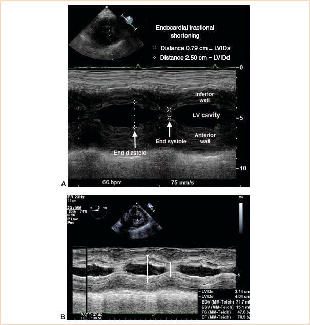
FIGURE 3.1 A: Transgastric mid short-axis view demonstrating M-mode measurements of ventricular cavity dimensions in systole and diastole using the leading edge to leading edge technique. LVIDd, left ventricular internal diameter at end diastole; LVIDs, left ventricular internal diameter at end systole; LV, left ventricular. B: Measurements made for the calculation of endocardial fractional shortening may also be used to calculate end diastolic volume, end systolic volume, and ejection fraction using the Cubed (Teichholz) formula.
The measurements required for this quantitative estimate of systolic function are LV internal diameter at end diastole (LVIDd, also called end diastolic diameter LVEDD) and LV internal diameter at end systole (LVIDs, also called end systolic diameter LVESD). These are measured from endocardial border to endocardial border (known as leading edge to leading edge) (2) from an M-mode tracing of a transgastric short-axis (TG SAX) view taken just above the papillary muscles (Fig. 3.1).
Although fractional shortening gives a rapid and simple estimate of LV systolic function, it is not a representative measurement in asymmetric ventricles such as those with regional wall abnormalities or aneurysmal deformation (1).
Left Ventricular Wall Thickness
Normal values: Men 0.6 to 1 cm, women 0.6 to 0.9 cm (1).
Measurements of LV wall thickness are made using the TG mid-SAX view. Usually both septal wall thickness at end diastole (SWTd) and posterior wall thickness at end diastole (PWTd) are reported. Septal wall thickness is measured from the right septal surface to the left septal surface, whereas posterior wall thickness is measured from epicardial surface to endocardial surface (being careful not to include pericardial tissue), using leading edge methodology for M-mode (2) and trailing edge to leading edge for 2D (1).
Relative Wall Thickness

Normal values: Men 0.24 to 0.42 cm, women 0.22 to 0.42 cm (1).
Relative wall thickness (RWT) is often used in patients with LV hypertrophy. In transesophageal echocardiography (TEE), the measurements are usually made in a TG SAX (just above the papillary muscles) and may be calculated from either of the two formulae given earlier. RWT is expressed as a decimal and used to describe LV hypertrophy and remodeling. An RWT equal to or greater than 0.42 denotes concentric hypertrophy (wall thickness is increased in the presence of a normal internal diameter) and an RWT less than 0.42 denotes eccentric hypertrophy (dilated internal ventricular dimension). The distinction between the two forms of hypertrophy is of prognostic interest, as concentric hypertrophy is associated with a higher incidence of cardiovascular events than eccentric hypertrophy.
Quantitative Evaluation of Left Ventricular Systolic Function—Planimetric Measurements
Area measurements offer improvements in accuracy over linear dimensions, as more of the LV is represented in the measurement.
Fractional Area Change

Normal values: Men 56% to 62%, women 59% to 65% (3).
The area of the LV cavity is measured at end systole (LVAs) and at end diastole (LVAd) and used to calculate fractional area change (FAC). Most commonly these measurements are made from the TG mid-SAX view of the LV, but when this view is suboptimal long-axis views can be substituted. The endocardium is manually traced around the LV cavity ignoring the papillary muscles.
Alternatively, automated border detection obviates the need to manually trace cavity area and provides real time, beat-to-beat measures of LVAd, LVAs, and FAC (Fig. 3.2). The acoustic properties of tissue and blood are discriminated because they create significantly different backscatter and thereby signal strength, allowing for automated detection of the endocardial border. A software package computes and displays the area of the LV (blood pool) cavity, superimposes it upon a 2D display of the ventricle and calculates the FAC on a beat-to-beat basis in the TG mid-SAX view. The echocardiographer adjusts the time-compensated gain, lateral gain, and overall gain settings to ensure that the displayed automated border tracks the endocardium throughout the cardiac cycle. For example, attenuation (or dropout) caused by the relative parallel orientation of myocardial fibers in the septal and lateral walls to the ultrasound beam in the SAX view decreases backscatter and therefore signal strength. Accordingly, adjustments to the lateral gain compensation are used to enhance receiver gain in these areas and allow for better tracking of the borders by the software.
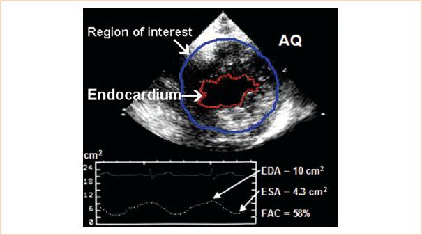
FIGURE 3.2 Transgastric mid short-axis view demonstrating automated border detection measurement (red line) of fractional area of change (lower panel ). AQ, acoustic quantification; EDA, end diastolic area; ESA, end systolic area; FAC, fractional area of change.
Quantitative Evaluation of Left Ventricular Systolic Function—Left Ventricular Volumes
LV volumes measured at end systole and end diastole are used to calculate ejection fraction. However, LV systolic volumes in and of themselves have prognostic value. Values greater than 70 mL are associated with increased risk for morbidity and mortality.
Left Ventricular Volume, Volumetric Equations Using Linear Measurements
There are a number of formulae in use which derive a three-dimensional (3D) LV volume from linear measurements. These are based on geometric models, which approximate the shape of a symmetric LV.
The Cubed formula (Teichholz method)
Cubed formula:

This formula assumes that the LV is approximated by a prolate ellipse, which has an SAX (minor axis, LVIDminor) equal to one-half of the long axis (or major axis, LVIDmajor) (Fig. 3.3). Measurement of the minor axis can be performed in the midesophageal (ME) two- or four-chamber or the TG two-chamber view and are taken at the mitral chordae level (1). Although the cube formula is the simplest formula, it compounds measurement errors because of the cube function and overestimates the volume of dilated ventricles. This occurs because the LV dilates primarily along the SAX, becoming more spherical in shape.
Volumetric Equations Using Planimetric Measurements
Again, these formulae are derived from geometric models which approximate a symmetrically shaped LV.
1. Single plane ellipsoid
Single plane ellipsoid method:

The LV volume is calculated assuming an ellipsoid shape. The long-axis diameter (LVIDmajor) and corresponding LV cavity area (LVALAX) obtained from a single long-axis view (ME four- or two-chamber, or TG two-chamber) are required for this formula (Fig. 3.4). The basal border of the LV cavity area is best delineated by a straight line connecting the mitral valve (MV) insertions at the lateral and septal borders of the annulus (1).
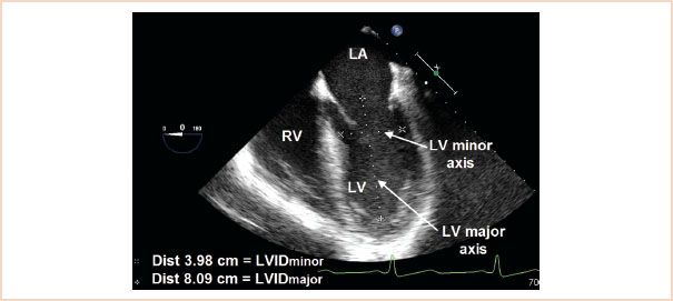
FIGURE 3.3 Midesophageal four-chamber demonstrating left ventricle (LV) as a prolate ellipse, which has a short axis (left ventricular internal diameter minor axis [LVIDminor]) equal to one-half of the long axis (or major axis LVIDmajor). The minor axis is used for the cubed formula. LA, left atrium; RV, right ventricle; LVID, left ventricle internal diameter.
2. Biplane ellipsoid
Biplane ellipsoid method:

This model incorporates the LV major axis diameter, LVIDmajor (acquired from an ME two- or four-chamber view or TG two-chamber view, which are all long-axis views) and the LV cavity area from the same image (LVALAX); plus the LV minor axis diameter (LVIDminor) acquired from the TG SAX of the LV view just above the papillary muscles; plus the corresponding LV cavity area from the same image (LVASAX).
3. Hemisphere–cylinder or bullet formula
Hemisphere-cylinder (or bullet formula):

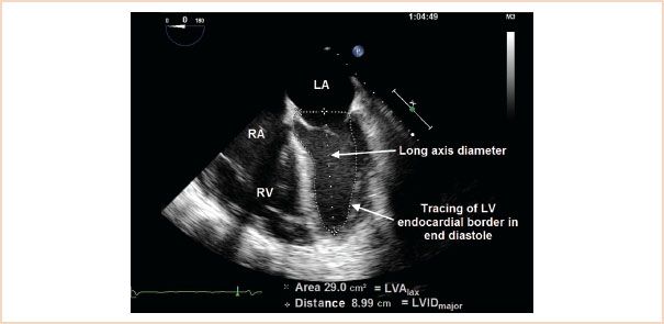
FIGURE 3.4 Midesophageal two-chamber demonstrating the measurements required for single-plane ellipsoid formula; a long-axis diameter (LVIDmajor) and the left ventricle (LV) area from the same long-axis view (LVALAX).·LA, left atrium; RA, right atrium; RV, right ventricle.
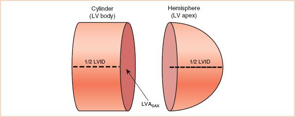
FIGURE 3.5 Demonstrates how the geometry of a cylinder plus a hemisphere approximates the left ventricle (LV) as a bullet. The length of the cylinder and the radius of the hemisphere are both equal to one-half of the left ventricular internal diameter major axis (LVIDmajor). LVASAX, left ventricle area from the short-axis view.
This model approximates the LV to the shape of a bullet (Fig. 3.5). Volume is calculated from a long-axis diameter (LVIDmajor) and the LV cavity area from the TG mid-SAX view (LVASAX). This formula is also known as the area length formula.
4. Method of disks (modified Simpson’s rule)
Modified Simpson’s rule:

In this method, the LV is described as a series of 20 disks from the base to the apex of the LV, like a stack of coins of decreasing size. The views required for this calculation are ME four- (Fig. 3.6) and two-chamber views. The computer software package calculates the volume of each disk as area × height and the volumes are summated to give a total LV volume. Foreshortening of the LV will result in underestimation of volume (1).
Since biplane planimetry (area acquired using both the ME four- and two-chamber views) corrects for shape distortion and minimizes mathematical assumptions, the method of disks is the recommended technique for volumetric measurements of the LV, particularly in those patients with regional wall motion abnormalities or an aneurysm (1). In cases where the endocardial border of the apex is not well seen, the area length method becomes the method of choice (1). Since it assumes a bullet-shaped LV, the area length method compensates for the inability to detect the apical endocardial borders.
Quantitative Evaluation of Left Ventricular Systolic Function—Left Ventricular Mass; Linear Measurements
All LV mass calculations are based on the subtraction of the volume of the LV cavity from the volume encompassed by the LV epicardium. This leaves LV myocardial volume, which is then multiplied by the density of myocardial tissue to calculate LV mass. The ASE recommends the following formula:

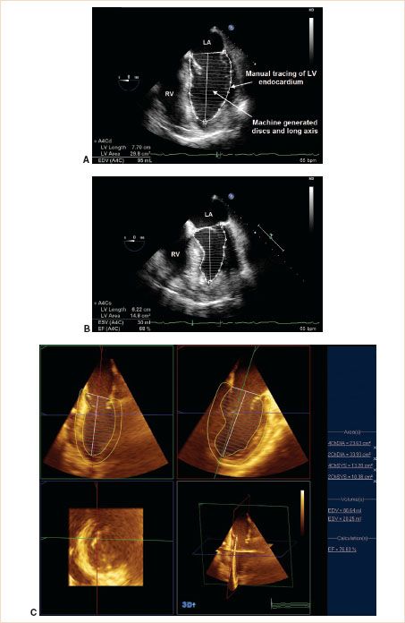
FIGURE 3.6 Midesophageal (ME) four-chamber views demonstrating the left ventricle (LV) measurements required for the method of disks (modified Simpson’s rule) to estimate LVEF. A: ME four-chamber view at end diastole; the endocardium is manually traced and the software calculates the LVIDmajor and divides the LV cavity into 20 discs. B: ME four-chamber view at end systole; the same measurements are made as in part A. These measurements are also required in the ME two-chamber view. Note that there should be less than a 10% discrepancy between the long-axis measurement of the ME four-chamber view in systole and the ME two-chamber view in systole (similarly in diastole). This ensures against foreshortening in one of the views. LA, left atrium; RV, right ventricle; EDV, end diastolic volume; ESV, end systolic volume; EF, ejection fraction. C: Three-dimensional echocardiography (3DE) may also be used for the calculation of left ventricular volumes, mass, and ejection fraction. The two views required (midesophageal two-chamber and midesophageal four-chamber) are generated simultaneously so that there will be no discrepancy between long-axis measurements.
TABLE 3.1 Normal Values for Echocardiographic Left Ventricular Systolic Parameters Published by the American Society of Echocardiography (ASE)
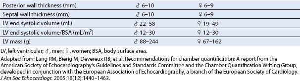
Increased LV mass is a stronger predictor than low ejection fraction (EF) for all-cause mortality and cardiac event rates in both hypertensive and normotensive populations. Since LV mass increases as a function of body size (except those with morbid obesity), LV mass is preferably expressed as a function of body surface area (BSA) (1). Normal values for LV mass are given as 67 to 162 g for women and 88 to 224 g for men. Indexed to BSA this becomes 43 to 95 g/m2 for women and 49 to 115 g/m2 for men (1) (Table 3.1). LV mass may be combined with RWT to categorize patients into various classes of hypertrophy (1) (see the following section on “Left Ventricular Hypertrophy”).
Quantitative Evaluation of Left Ventricular Systolic Function—Left Ventricular Mass, Planimetric Measurements
In the determination of LV mass using planimetric measurements, either the area length method or the truncated ellipsoid method are recommended (1,4). Most current echocardiography machines include the software to calculate LV mass by one or both of these two methods. The LV is acquired in the TG mid-SAX view. An area tracing is made of the epicardial and endocardial borders. The difference between the two areas is the area occupied by the myocardium. A major axis length is then acquired from a long-axis view and the software calculates the mass of the LV according to the formulae used by the vendor (1,4) (Fig. 3.7).
Quantitative Evaluation of Left Ventricular Systolic Function—Rate of Ventricular Pressure Rise
The rate of rise in ventricular pressure (dP/dT) has been demonstrated to be well correlated with systolic function. The greater the contractile force exerted, the greater the rise in ventricular pressure. Previously, this could only be measured invasively with LV catheterization; however, continuous wave Doppler (CWD) determination of the velocity of a mitral regurgitant (MR) jet allows calculation of instantaneous pressure gradients between the left ventricle and the left atrium (LA). Left atrial pressure variations in early systole can be considered to be negligible; therefore, the rising segment of the MR velocity curve during isovolumetric contraction should essentially reflect LV pressure increase only. If the rate of rise in ventricular pressure is reduced because of poor LV function, the rate of increase of the MR jet velocity will also be low.
To perform a dP/dT measurement (Fig. 3.8), the MR jet is interrogated with CWD. The cursor is placed on the MR velocity profile at 1 m/s and then at 3 m/s and the time interval between the two points is determined (5). Using the simplified Bernoulli equation, the pressure differential is [4(3)2] − [4(1)2] or 32 mm Hg. dP/dT is therefore 32 mm Hg divided by the time interval in seconds. Normal values exceed 1,000 mm Hg/s.
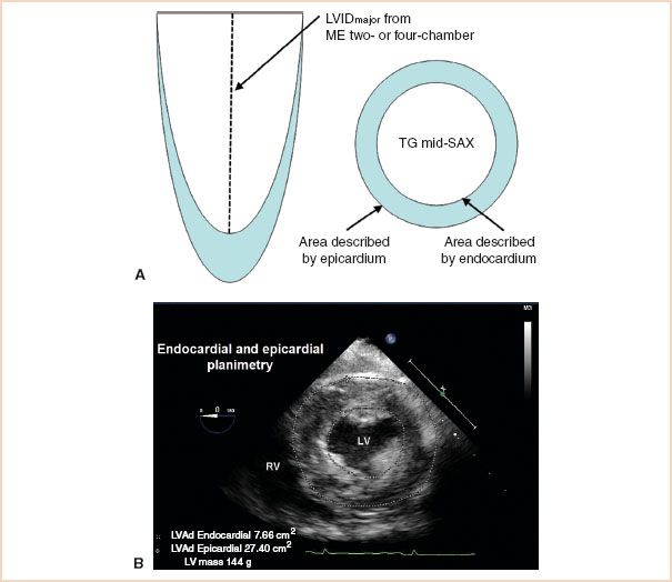
FIGURE 3.7 Left ventricular (LV) mass calculation. A: Diagram representing the views and measurements required for planimetric LV mass calculation. B: The endocardium and epicardium are traced in the transgastric mid short-axis view and the software calculates LV mass using left ventricular internal diameter major axis (LVIDmajor) (from a long-axis view as in part A) and density of myocardial tissue. LVAd, area of left ventricular cavity measured at end systole.
Newer Echocardiographic Modalities for Assessing Left Ventricular Systolic Function
Three-dimensional Echocardiography
The advent of three-dimensional echocardiography (3DE) has revolutionized the acquisition and understanding of echocardiographic data. Currently there are two methods of acquiring 3DE images. One technique utilizes a set of 2D images which are then used to reconstruct the 3D image. This method requires an “offline” reconstruction. Limitations of this form of 3DE include time for reconstruction and the need for a regular cardiac rhythm during the acquisition period. The second technique employs a matrix array transducer, which scans a pyramidal-shaped sector and displays the image in real time. Using this technology, 3DE images of the LV can be acquired over one beat and displayed in real time (6).
The advantage of 3DE for measuring LV volumes and masses is that the LV can be acquired and displayed in its true shape avoiding the need for mathematical modeling. This means that regional function can be included in the overall estimates, producing a more accurate measurement (Fig. 3.9, Video 3.1). Furthermore, inaccuracies do not occur because of plane positioning errors and foreshortening. Three-dimensional echocardiography is highly correlated with the gold standard of imaging (magnetic resonance imaging [MRI]), producing a better agreement with lower inter- and intraobserver variations than 2DE in normal subjects (7) and patients with regional wall motion abnormalities (8).
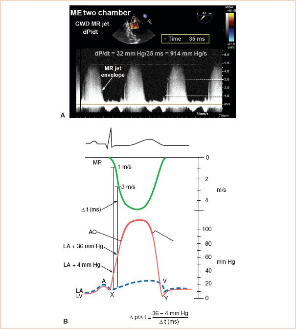
FIGURE 3.8 A: Calculation of dP/dT. Place caliper on mitral regurgitant (MR) jet envelope at 1 m/s and again at 3 m/s to measure the time for the instantaneous pressure gradient between the left ventricle (LV) and left atrium (LA) to rise from 4 mm Hg to 36 mm Hg. B: Upper panel—electrocardiography (ECG); middle panel—Doppler trace of MR jet (acquired from transthoracic approach); lower panel—equivalent pressure recordings at catheterization. CWD, continuous wave Doppler. (Part B from Pai RG, Bansal RC, Shah PM. Doppler-derived rate of left ventricular pressure rise. Its correlation with the postoperative left ventricular function in mitral regurgitation. Circulation. 1990;82(2):514–520.)
Visual display of 3D systolic performance varies from vendor to vendor. The LV may be displayed as raw images, a wire framework, or a reconstructed volumetric figure in which the walls of the LV can be visualized according to the American Heart Association (AHA)/ASE 17-segment model (Fig. 3.9, Video 3.1). The contribution of each segment to volume and mass can be displayed as individual waveforms enabling an assessment of global and regional performance from one image. Data can also be displayed as color-coded representations of regional LV segmental excursions superimposed on the standard “bull’s eye” display (Fig. 3.9B) assisting visualization of regional function.
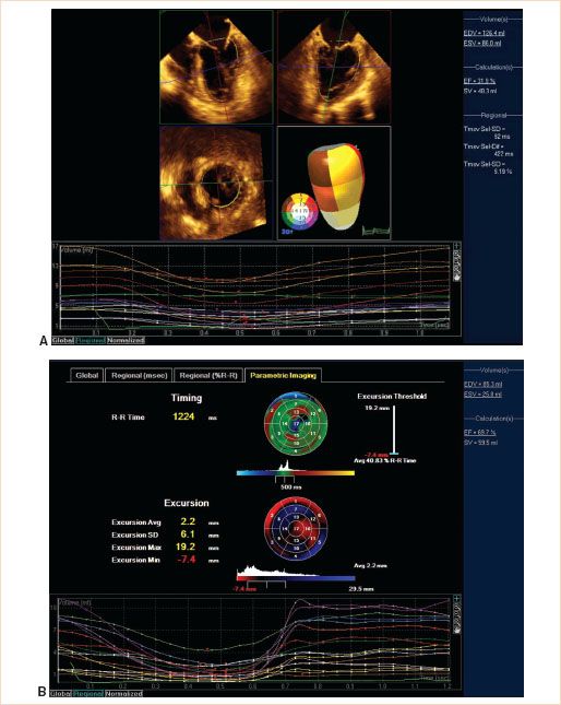
FIGURE 3.9 A: Three-dimensional (3DE) echocardiography. Top panels: Midesophageal (ME) four- and two-chamber views. Middle panels: Transgastric short-axis view and AHA/ASE 17-segment volumetric model. Bottom panel: Individual segment contribution to overall left ventricular volume throughout the cardiac cycle. B: Mapping data from 3DE of left ventricle with an anterior aneurysm. Upper panel: Timing of onset of contraction related to the mean value which is depicted in green. Red denotes delayed contraction, blue denotes early contraction. Middle panel: Excursion of individual segments toward the center of the left ventricle (LV). Blue denotes movement toward the center, black denotes no movement (akinesia), and red denotes movement away from the center (dyskinesia). Color brightness denotes extent of movement. Lower panel: Individual segment contribution to LV volume. See Figure 3.9(A) for color coding of the individual segments. See also Video 3.1.
Tissue Doppler Imaging
The high temporal resolution of Doppler imaging is specifically suited to the accurate measurement of velocities at precise locations in the heart. When Doppler is used in its original application to measure blood flow, high-pass filters are employed to screen out the low velocities from the myocardium, valvular structures, and vessel walls. In contrast, tissue Doppler imaging (TDI or tissue Doppler echocardiography, TDE) measures the velocity of myocardial tissue using low-pass filters to screen out higher velocities generated by blood flow. Unlike blood flow Doppler signals that are typified by high velocity and low amplitude, myocardial motion is characterized by low velocity and high amplitude. Tissue motion creates Doppler shifts that are approximately 40 dB higher than Doppler signals from blood flow and their velocities rarely exceed 20 cm/s. To record low wall motion velocity, gain amplification is reduced and high-pass filters are bypassed.
During image acquisition, it is important to optimize temporal resolution by selecting as narrow an image sector as possible, which increases frame rate (>150/s is recommended, Fig. 3.10). Equally important is to select the appropriate velocity scale. These parameters should be optimized at the time of imaging, as it is not possible to modify the frame rate and the velocity scale during postprocessing image analysis.
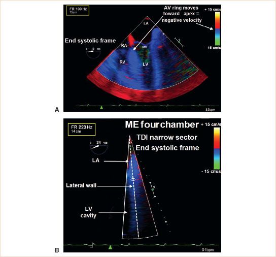
FIGURE 3.10 Tissue Doppler imaging (TDI). A: TDI of a midesophageal (ME) four-chamber view acquired as a full-sector view; frame rate is 100 Hz. B: The same image is acquired but the sector is narrowed down to improve frame rates. Note that frame rates have increased from 100 Hz to 223 Hz. LA, left atrium; RA, right atrium; MV, mitral valve; RV, right ventricle; LV, left ventricle.
In TDI, a small pulsed wave sampling volume measures the velocities of the myocardium as it moves toward and away from the transducer. The sample volume is placed in the middle of a segment of the heart and velocities within that area are measured. A velocity against time plot is displayed, using the convention that tissue moving toward the transducer is positive. For example, during interrogation of the basal segment of the septum in the ME four-chamber view, as the heart contracts and thickens during systole the atrioventricular ring moves toward the apex and thereby will move away from the transducer producing a negative deflection.
Since this is a Doppler technique, TDI will underestimate the myocardial velocities if the angle of interrogation is not parallel to motion (9). Although most ultrasound platforms allow for correction of the Doppler equation for the angle of incidence, this is not recommended (7). Rather, it is recommended that for an ME view, the wall to be interrogated is placed in the center of the imaging sector to better align the angle of interrogation (Fig. 3.10).
Other errors encountered using TDI are caused by tethering as velocity imaging is confounded by velocities from adjacent segments. For example, in an ME four-chamber view, an akinetic segment at the basal part of the septum should by definition have a longitudinal systolic velocity of zero. However, if the midventricular segment of the septal wall moves normally, the tethering effect will cause the akinetic basal segment to move longitudinally.
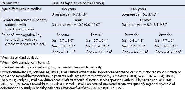
In general, longitudinal measurements are made of the basal and midventricular segments, obtained from the ME two- and four-chamber views. A gradient of systolic velocities exists from the base of the heart to the apex. Peak systolic longitudinal velocities at the MV annulus (Sa) are greater compared to those at the midventricular segments (Sm). Sm velocities are more representative of overall systolic function. Annular velocities are difficult to acquire in patients with mitral annular calcification or with a prosthetic valve or annuloplasty ring. Myocardial velocities are age and gender dependent (Table 3.2). From transthoracic studies, patients with normal global LV function have systolic velocities greater than 7.5 cm/s (10), whereas velocities less than or equal to 5.5 cm/s indicate LV failure (11). Systolic velocities less than 3 cm/s are associated with a significantly increased risk of cardiac death within 2 years (12). (Note that values are positive because transthoracic measurements are acquired from the apex of the heart.)
The typical systolic TDI profile (Fig. 3.11) has two parts with a biphasic wave during isovolumic contraction (IVCa and IVCb) and a monophasic wave during systolic ejection. IVCa corresponds to the timing of the MV closure and represents early myocardial activation at the base of the heart, occurring 20 to 30 milliseconds earlier in the anteroseptal than the posterior free wall (13). The movement of the myocardium at the annulus is inward and toward the apex. The second wave IVCb is in the opposite direction caused by subsequent contraction of the apex making the base bulge up and outward just before ejection. The monophasic systolic wave is directed inward and toward the apex and represents contraction of the LV during ejection.
TABLE 3.2 Factors Affecting Tissue Doppler Imaging Velocity Measurements
Related posts:
 A Practical Approach to the Echocardiographic Evaluation of Ventricular Diastolic Function
 Prosthetic Valves
Stay updated, free articles. Join our Telegram channel

Full access? Get Clinical Tree


