2Linear models with classical error In this chapter, we illustrate the problems arising when estimating regression parameters with classical measurement errors using an example of the simplest regression model, the linear one. It is described by the following two equations: All the variables are scalar. This model has been used in an example of Section 1.1. Here ξi is unobservable value of the latent variable (the ξi acts as a regressor), xi is the observed surrogate data, yi is the observable response, εi is the response error, and δi is the measurement error in the covariate. We have to estimate the intercept β0 and the slope β1. Typical are the following assumptions about the observation model. (i)Random variables ξi, εi, δi, i ≥ 1, are independent. (ii)The errors εi are identically distributed and centered with finite and positive variance (iii)The errors δi are identically distributed and centered with finite and positive variance In the structural case, the latent variable is random. Or speaking more precisely, we require the following: (iv)Random variables ξi are identically distributed, with Eξi = μξ and Note that under conditions (i) and (iv), the random variables ξi are independent and identically distributed. In the functional case, the next condition holds instead of (iv). (v)The values ξi are nonrandom. We try to transform the model (2.1) and (2.2) to an ordinary linear regression. Excluding the ξi from equation (2.1) we have The model (2.3) resembles an ordinary linear regression, with errors τi. Given (i)–(iii), the random variables τi are centered, independent, and identically distributed. We get As we can see, the new error variance depends on the slope β1. This is the first difference of the model (2.3) from the ordinary regression, where usually the error variance does not depend on regression parameters. Thus, in case of β1 ≠ 0 (i.e., when in equation (2.1) there is a real dependence between the response and regressor ξi), we have Inequality (2.6) is the second main difference of the model (2.3) from the ordinary regression, where it is strictly required that the regressor and the error are uncorrelated. One can see that in essence the model (2.1) and (2.2) does not come to the ordinary regression. Therefore, the theory of linear measurement error models is substantial. In the following the structural errors-in-variables model with assumptions (i)–(iv) will be mainly under consideration. Choose Θ = R2 in the model (2.1) and (2.2) as a parameter set for the augmented regression parameter β = (β0,β1)T. Such a choice of Θ corresponds to the absence of a prior information about possible values of regression parameters. According to Section 1.4.1, the naive estimator Therefore, Find an explicit expression for the naive estimator. Denote the sample mean as Hereafter bar means averaging, e.g., The sample variance of the values xi is defined by the expression and the sample covariance between xi and yi by the expression There are other useful representations of the statistics (2.11) and (2.12): Theorem 2.1. In the model (2.1) and (2.2), let the sample size n ≥ 2, and moreover, not all the observed values xi coincide. Then the objective function (2.7) has a unique minimum point in R2, with components Proof. A necessary condition for It has the form Eliminate Since not all the values xi coincide, Sxx ≠ 0. Hence, Thus, if a global minimum of the function QOLS is attained, then a minimum point is The function QOLS is a polynomial of the second order in β0 and β1. This function can be exactly expanded in the neighborhood of The derivative The matrix S is positive definite, because S11 = 1 > 0 and det This proves (2.20) and the statement of the theorem. Remark 2.2. Based on the naive estimator, one can draw a straight line The line will pass through the center of mass M ( Study the limit of the naive estimator, as the sample size grows. Here we consider the structural model. Recall that the reliability ratio Theorem 2.3. Given (i)–(iv), it holds that Proof. Using the strong law of large numbers (SLLN), we find limit of the denominator of expression (2.14): Therefore, the statistic Sxx becomes positive with probability 1 at n ≥ n0(ω) (i.e., starting from some random number); then one can apply Theorem 2.1. Again by the SLLN, Here, random variables (x, ξ, δ, ε, y) have the same joint distribution as (xi, ξi, δi, εi, yi). As ξ, δ, ε are jointly independent, we have further Thus, with probability 1 at n ≥ n0(ω) it holds that The theorem is proved. Relation (2.25) shows that the estimator In particular, using the naive estimator in the binary incidence model (1.2), (1.4), and (1.5) leads to the attenuation of dependence of the odds function λ on the exposure dose ξi: thus, we will have with the estimated excess absolute risk (EAR) Now, it is required that the latent variable and the measurement error be normally distributed. Thus, we specify the conditions (iii) and (iv). (vi)The errors δi are identically distributed, with distribution (vii)Random variables ξi are identically distributed, with distribution The conditions (i), (ii), (vi), and (vii) are imposed. The prediction problem in the model (2.1) and (2.2) is the following: if the next observation xn + 1 of the surrogate variable comes, the corresponding observation yn + 1 of the response should be predicted. The optimal predictor From probability theory, it is known that such an optimal predictor is given by the conditional expectation: The vector (yn + 1, xn + 1)T is stochastically independent of the sample y1, x1,…, yn, xn, therefore, Since εn + 1 and xn + 1 are independent, we have Further, using the normality assumptions (vi) and (vii) we can utilize the results of Section 1.4.3 and get Equalities (2.32) – (2.34) yield the optimal predictor At the same time, this predictor is unfeasible because the model parameters β0, β1, K, μξ are unknown. Relying on the naive estimator one can offer the predictor Unexpectedly, this predictor is little different from Theorem 2.4. Assume (i), (ii), (vi), and (vii). Then Therefore, the predictor (Hereafter o(1) denotes a sequence of random variables which tends to 0, a.s.) Proof. The convergence (2.38) follows from Theorem 2.3. Consider whence (2.37) follows. Thus, we finally have The theorem is proved. Interestingly, a consistent estimator Indeed, we would then construct a predictor which at large n, approaches to β0 + β1 xn + 1 that is significantly different from the optimal predictor (2.35). The reason for this phenomenon is as follows: The precise estimation of model coefficients and accurate prediction of the next value of the response feedback are totally different statistical problems. The more so as we need a prediction based on the value xn + 1 of the surrogate variable rather than the value ξn + 1 of the latent variable. In the latter case the next conditional expectation would be the unfeasible optimal predictor: and then the predictor In Section 2.2, random variables ξi and δi were normal but εi was not necessarily. Now, consider the normal model (2.1) and (2.2), i.e., the εi will be normal as well. (viii)Random variables εi are identically distributed, with distribution In this section, we solve the following problem: In the model (2.1) and (2.2), assume the conditions (i) and (vi) – (viii) are satisfied; is it possible to estimate the parameters β0 and β1 consistently if the nuisance parameters In total, we have six unknown model parameters that fully describe the distribution of the observed normal vector (y; x)T. Let us give a general definition of a not identifiable observation model. Let the observed vectors be


 .
.
 .
.
 .
.


2.1Inconsistency of the naive estimator: the attenuation effect
 naive =
  OLS is defined by minimizing in R2 the objective function


 to be the minimum point of the function QOLS is the so-called system of normal equations:


 0 from the second equation:


 = (
= ( 0,
0,  1)T from (2.19). Now, it is enough to show that

 using Taylor’s formula

 because
  satisfies (2.15), and the matrix of the second derivatives
  does not depend on the point where it is evaluated:

 Therefore, at β ≠
  from (2.21), we have


 ,
,  ) of the observed points Mi(xi; yi),
  . In fact, it follows from the first equation of system (2.16). The line (2.24) is an estimator of the true line y = β0 + β1 ξ in the coordinate system (ξ; y).
 has been introduced in Section 1.4.3. The almost sure (a.s.) convergence is denoted by
  .
.


 naive is not consistent, because for
  1 ≠ 0, the estimator β1, naive does not converge in probability to β1 (in fact, it converges a.s., and therefore, in probability, to Kβ1 ≠ β1). The phenomenon that the limit of the slope estimator is the value Kβ1 located between 0 and β1, is called attenuation effect. It characterizes the behavior of the naive estimator in any regression model with the classical error. The effect is plausible by the following argument. Consider the predictive line (2.24). Thanks to the convergence (2.25), the slope of the line is close to Kβ1 at large n. If β1 ≠ 0 and n is large, the line (2.24) passes more flat than the true line y = β0 + β1 ξ. Thus, we conclude that the estimated dependence y of ξ is weaker than the true one.

 1, naive < β1. It should be noted that the latter inequality will hold at sufficiently large sample size.
2.2Prediction problem

 n + 1 is sought as a Borel measurable function of the sample and the value xn + 1, for which the mean squared error E(ŷn + 1 – yn + 1)2 is minimal.


 n + 1, for large n.


 n + 1 is close to the optimal one


 is worse applicable to the prediction problem.


 0 +
0 +  1 ξn + 1 based on the consistent estimator would be more accurate than the predictor
  0, naive +
  1, naive · ξn + 1 (see Remark 2.2).
2.3The linear model is not identifiable
 and
and 
 are unknown?

Related posts:
 Overview of risk models realized in program package EPICURE
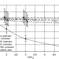 Estimation of radiation risk under classical or Berkson multiplicative error in exposure doses
 Radiation risk estimation for persons exposed by radioiodine as a result of the Chornobyl accident
Stay updated, free articles. Join our Telegram channel

Full access? Get Clinical Tree


