LV Feature Detection and Blood-Pool Tracking from Multi-plane TEE Time Series

to one another) TEE image sequences through the cardiac cycle to validate the proposed tools and demonstrate their clinical utility and performance against commercial, clinical-grade, clinician-operated software.

The proposed methodology encompasses three steps: (1) endocardial left ventricle (LV) feature extraction and blood-pool segmentation from the raw 2D multi-plane image sequences, (2) frame-to-frame feature tracking and propagation through the cardiac cycle using non-rigid image registration, and (3) 3D reconstruction of the LV blood pool geometry at the desired cardiac phases using spline-based interpolation and convex hull fitting.

2.1 LV Feature Extraction and Blood-Pool Segmentation

Image Pre-processing via Monogenic Filtering: Unlike intensity-based edge detection algorithms are inefficient in identifying features from US images, intensity invariant local phase-based techniques have shown promising results [10], where a local phase of $\pm \pi /2$ signifies high symmetry, while a local phase of 0 or $\pi$ signifies high asymmetry [12]. The local phase computation of a 1D signal uses a complex analytic signal comprised of the original signal as the real part and its corresponding Hilbert transform as the imaginary part. However, since the Hilbert transform is mathematically restricted to 1D with no straightforward extension to 2D and 3D, we used the method described in [13] to extend the concept of the analytic signal to higher dimensions using a monogenic signal. The higher dimension monogenic signal is generated by combining a bandpass Gaussian-derivative filter with a vector-valued odd filter (i.e., a Reisz filter). The low frequency variations in the local phase are extracted using a high spread ( $\sigma$ ) Gaussian-derivative filter, while the high frequency components are extracted using a low spread ( $\sigma$ ) Gaussian-derivative filter. The described monogenic filtering sequence is used to transform each of the three tri-plane 2D US images into corresponding “cartoon” images in which the blood pool and myocardial wall appear enhanced, facilitating their segmentation in the subsequent step.

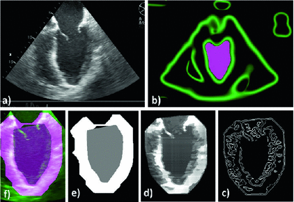
Fig. 1.

Segmentation Workflow: (a) original US image, (b) high spread ( $\sigma$ ) low frequency monogenic filter applied to the “2D + time” image dataset shown with the high confidence blood pool mask, (c) low spread ( $\sigma$ ) high frequency monogenic filter output with blood pool removed, (d) “cartoon” image with enhanced regions, and (e) graph cut segmentation output (f) superimposed onto the original image.

Graph Cut-Based Segmentation: The resulting “cartoon” image is used to construct a four neighborhood graph structure in which each pixel is connected to its east, west, north and south neighbors. Three special nodes called terminals are added, which represent three classes (labels): background, blood pool and myocardium. The segmentation can be formulated as an energy minimization problem to find the labeling f, such that it minimizes the energy:

$\begin{aligned} E(f)~=~\sum \limits _{\{p,q\} \in \mathcal {N}} V_{p,q}(f_p,f_q)~+~\sum \limits _{p \in \mathcal {P}} D_p(i_p,f_p), \end{aligned}$

(1)

where the first term represents smoothness energy, which forces pixels p and q defined by a set of interacting pair $\mathcal {N}$ , towards the same label. The second term represents the data energy that reduces the disagreement between the labeling f and the observed data

. The links between each pixel and the terminals (i.e., t-links) are formulated as the negative logarithm of the normal distribution [14]:

$\begin{aligned} D_p(i_p,f_p)=-ln\left( \frac{1}{\sigma \sqrt{2 \pi }}exp\left( -\frac{(i_p-\mu )^2}{2 \sigma ^2}\right) \right) , \end{aligned}$

(2)

where $\mu$ and $\sigma$ are the mean and standard deviation for the three classes obtained from the image. The links between neighboring pixels, called n-links, are weighted according to their similarity to formulate the smoothness energy:

$$$\begin{aligned} V_{p,q}(f_p,f_q) = {\left\{ \begin{array}{ll} 2K \cdot T(f_p \ne f_q) &{} \text {if}~|I_p-I_q| \le C\\ K \cdot T(f_p \ne f_q) &{} \text {if}~|I_p-I_q| > C \end{array}\right. } \end{aligned}$$” src=”/wp-content/uploads/2016/09/A339585_1_En_4_Chapter_Equ3.gif”></DIV></DIV><br /> <DIV class=EquationNumber>(3)</DIV></DIV>where <SPAN id=IEq12 class=InlineEquation><IMG alt=$ is 1 if its argument is true, and otherwise 0, K is a constant, and C is a intensity threshold that forces the neighboring pixels within the threshold towards the same label. The minimum cut equivalent to the maximum flow is obtained via the expansion algorithm in [11] yielding optimal segmentation of background, blood-pool, and myocardium (Fig. 1e).

2.2 Frame-to-frame Feature Tracking and Propagation

Image Pre-processing: Once a single-phase image is segmented using the procedure outlined in Sect. 2.1, the extracted features are tracked and propagated throughout the cardiac cycle using non-rigid registration (Fig. 2). Prior to registration, each “2D + time” image sequence corresponding to each of the tri-plane views is first “prepared” by identifying a region of interest-based “bounding box” centered on the features that belong to the LV. To ensure the chosen “bounding box” spans the entire LV including blood-pool, myocardium, and surrounding region, this window is selected based on the high confidence blood pool mask obtained after the application of the high spread Gaussian-derivative filter employed in Sect. 2.1 to the entire image sequence, followed by an isotropic dilation to ensure full coverage beyond the LV myocardial boundary. Moreover, the mitral valve region is “trimmed” using a straight line joining the leaflet hinges.

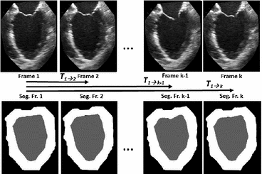
Fig. 2.

The frame-to-frame motion transforms ( $T_{(k-1)\rightarrow k}$ ) are estimated by non-rigidly registering adjacent images in the sequence, then concatenated ( $T_{1\rightarrow k}$ = $T_{1 \rightarrow 2}$ $\cdot$ … $\cdot$ $T_{(k-1) \rightarrow k}$ ) and applied to the segmented end-diastolic (ED) frame ( $F_{k}$ = $T_{1 \rightarrow k}$ $\cdot$ $F_{1}$ = $T_{(k-1) \rightarrow k}$ $\cdot$ … $\cdot$ $T_{1 \rightarrow 2}$ $\cdot$ $F_{1}$ ).

Non-rigid Registration Algorithm: The employed registration algorithm is a modified version of the biomechanics-based algorithm proposed by Lamash et al. [15]. The LV anatomy is modeled as a two compartment model consisting of muscle — linear elastic, isotropic, and incompressible, and blood-pool, with prescribed smoothness constraints to allow rapid motion of the endocardial contour. We initialize the algorithm by first discretizing the endocardial and epicardial contours, then constructing a mesh of the blood-pool and myocardium. Rather than resorting to a rectangular grid, we account for the local curvature of the endocardial border using a finite-element like mesh defined via linear shape functions. The algorithm deforms the mesh by estimating the required deforming forces that minimize the sum of the squared difference between the initial and target images (Fig. 3). To avoid large deformations and ensure a smooth displacement field, a linear elastic regularization approach [16] is utilized.

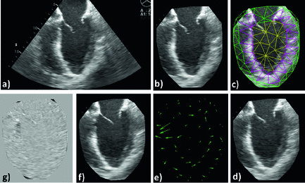
Fig. 3.

Registration workflow: (a) the original image is “prepared” by automatically identifying an LV-centered ROI (b) onto which the mesh is applied (c), then registered to the target image (d); the resulting displacement field (e) is applied to the pre-registered image (b) to obtain the registered image (f), which can be compared to the target image (d) by visualizing the digitally subtracted image (g).

2.3 3D LV Volume Reconstruction

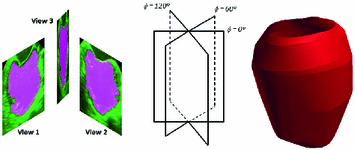
Following the segmentation of each of the tri-plane views at end-diastole using the technique in Sect. 2.1 and their propagation throughout the cardiac cycle, the resulting images are re-inserted into a pseudo-3D image volume along the same orientation at which they were originally acquired (i.e., 60 $^\circ$ apart) corresponding to each cardiac phase. The boundary points of each segmented contour at the same elevation are then fitted using the parametric variational cubic spline technique in [17]. The spline interpolated data is used to generate a convex hull using the algorithm proposed in [18] (Fig. 4).

Fig. 4.

Schematic illustration of the 3D LV reconstruction: the tri-plane views at 60 $^\circ$ (a) are inserted at their appropriate orientation (b), followed by spline interpolation and convex hull generation (c).

3 Evaluation and Results

We conducted a preliminary study using retrospective tri-plane time series data spanning multiple cardiac cycles from patients who underwent TEE imaging for cardiac function assessment. Since the proposed framework encompasses three different components — automatic extraction of endocardial features, registration-based feature tracking and propagation, and volume reconstruction — we assessed the performance of each component against the ground truth, which consists of the blood-pool representation annotated manually by the expert clinician, using the EchpPac PC clinical software. In addition, we also evaluated the performance at each stages of our application running in MATLAB on an Intel $^\circledR$ Xenon $^\circledR$ 3.60 GHz 32 GB RAM PC.