Magnetism is a property of matter. It results from electrons orbiting around atoms, and these spinning electrons cause the atom to have a magnetic moment. The magnetic field strength is measured in units of gauss (g) and tesla (T). One tesla is equivalent to 10 000 gauss. The earth’s magnetic field, which is strong enough to keep us from drifting into space, is about 0.5 g. The typical magnetic resonance imaging (MRI) machine produces a field strength of 1.5 T.
MRI is a technique for generating a cross-sectional image of the body based on magnetic resonance of atomic nuclei, rather than on the passage of ionizing radiation as with computed tomography (CT). MRI offers several advantages over CT for orbital imaging:
- •
Because of the near absence of resonance signal generated from bone in MRI, soft tissue visualization in the region of the orbital apex, optic canal, and cavernous sinus is not degraded by dense surrounding bone as in CT scans.
- •
Manipulation of resonance signals from various tissues provides contrast variability and tissue differentiation unobtainable with any X-ray technique.
- •
Surface coil technology, improvements in signal-to-noise ratios (SNRs), and techniques for suppressing the high fat signal have vastly improved visualization of orbital lesions.
- •
MRI has proven especially valuable for intracranial lesions in the vicinity of the optic chiasm and suprasellar cistern, and has all but replaced older techniques.
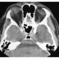
Some tissues cannot be evaluated with MRI. Because MR signals are generated only from mobile protons, those tightly bound in bone do not produce a resonance signal and therefore bone appears black. Similarly, air contains very few protons, and it also appears black. If bone is of clinical interest, or details of the bone–air/tissue interface are important, then CT should be used in addition to MRI.
The MRI system consists of a number of components:
- •
A large magnet to generate the external magnetic field
- •
Shim coils to help correct any inhomogeneities in the field
- •
A radiofrequency (RF) coil to transmit a radio signal to the imaged tissue
- •
A receiver coil to detect the returning radio MR signals
- •
Gradient coils to provide spatial localization
- •
A computer to reconstruct the signals into a final MR image.
Physics of magnetic resonance imaging
The major component of the MRI system is the magnet that provides the primary polarizing field. This is usually a set of coils of superconducting wire suspended in liquid helium. The quality of the MR image generally increases with the field strength, measured in tesla units. Most clinical systems operate at about 1.5 T. Located within the bore of the magnet are gradient coils, which provide the spatial localization information during the imaging process. Within the gradient coils are the RF antennae (‘coils’), which transmit the RF energy to the tissues and receive the returning resonance signals. The use of smaller surface coils placed immediately over the area of interest increases the signal strength and decreases the SNR. These permit the acquisition of the high-resolution images of modern scanners. However, such coils are limited in the depth of penetration they can image, and they are associated with some artifacts.
Magnetic resonance imaging depends upon the presence of magnetic isotopes of common elements in biologic tissues. These are atomic nuclei containing an odd number of protons and/or neutrons, such as 1 H, 13 C, 14 Na, 23 N, and 31 P. The unpaired proton has spin and confers a net magnetic field. In nuclei where all the protons are paired, the magnetizations cancel each other out. Because the resonance signal from each atom is so very small, the sum of many atoms must be used to generate an adequate image. In biologic tissues, the hydrogen atom, or proton, is ubiquitous and therefore medical MRI utilizes hydrogen as the resonating nucleus of interest. Although the associated electron can undergo a spin resonance similar to that of the nucleus, it does not contribute to the MR signal.
The nucleus of a hydrogen atom consists of a single proton having a positive charge, with one electron having a negative charge orbiting around it ( Figure 2.1 ). Like most elemental particles, protons have what is called ‘spin’. This is a quantum mechanical property of such particles. It is not exactly the same as the concept of a spinning particle which rotates around an axis like a spinning top. Nevertheless, it is useful to think about it in such terms. Because the proton has a small mass ( m ), its rotational movement can be described as angular momentum ( L ) ( Figure 2.2 ). Angular momentum of a spinning particle about a given origin is defined as:
L = r × p
- •
L is the angular momentum of the particle
- •
r is the position vector of the particle from the origin
- •
p is the linear momentum of the particle.


The angular momentum is constant for any particular species of atomic particle, such as a proton. Unlike a top whose spin ultimately slows down and stops because of friction with the floor, the proton’s spin is a basic property and, therefore, is a conserved quantity. The angular momentum can be transferred by an external torque, but otherwise can be neither increased nor decreased. Being a charged particle, the rotating proton produces a current loop around its axis of spin, and this in turn induces a magnetic field with north and south poles aligned with the spin axis like a bar magnet. This is referred to as a magnetic dipole moment, or just magnetic moment ( B ) ( Figure 2.3 ). The dipole moment can produce magnetic interactions with its environment. Thus, when the spinning proton passes through an external magnetic field or is affected by an electromagnetic wave, it can induce a voltage in a receiver coil.

In tissue not acted upon by an external magnetic field the many different spinning protons have no uniform orientation ( Figure 2.4 ). The axes of rotation are randomly oriented in space canceling each other out, and therefore there is no net magnetic moment. The Earth’s gravitational field is too weak to have a significant effect on them. However, when placed within a strong static external magnetic field (B 0 ), the parent molecules within which the protons reside undergo thermal movement and this energy slowly causes slight changes in the magnitude and direction of the magnetic moments. The moments of the spinning protons gradually align themselves with the external field direction, just like the needle of a compass aligns itself with the Earth’s weak magnetic field ( Figure 2.5 ).


In addition to aligning with the external magnetic field, the upper pole of the magnetic moments exhibit a wobble around the external magnetic direction, much like the axis of a top describes a cone as it spins around the direction of gravitational force ( Figure 2.6 ). This wobble is called precession and its rotational speed is proportional to the external magnetic field strength. This speed is called the Larmor frequency , which is defined as:
ω 0 = γ 0 × B 0
- •
ω 0 is the Larmor frequency
- •
γ 0 is the gyromagnetic ratio which is a constant specific to each atomic particle species, and
- •
B 0 is the strength of the external magnetic field measured in tesla (T).

For protons, the gyromagnetic ratio is 42.58 MHz/T so that at a magnetic strength of 1.5 T MRI the Larmor frequency is 63.87 MHz, and at 3 T it is 127.7 MHz.
As the magnetic moments align themselves with the external magnetic field they establish a net longitudinal magnetization along the z-axis as the individual magnetic moments are added together ( Figure 2.7 ). The strength of this magnetization represents the sum of the individual moments. However, the spins can align either parallel or antiparallel to the external field direction, with a slight preference for the parallel orientation because it represents a lower more favorable energy state. Thus, once the system has reached a steady-state thermal equilibrium, this slight preponderance of + orientations results in a net magnetization, M z , along the z-axis. Because this lies parallel to the external field direction it is also referred to as longitudinal magnetization . Most of the magnetic moments are not perfectly aligned with the z-axis, but lie at various small angles to it as they precess. Also, they are equally distributed 360° around it.

This stable system, with spin moments precessing around B 0 can now be acted on by energy from the outside. In MRI this is achieved with an electromagnetic (RF) radio wave. If this RF wave is delivered along the x- or y-axis oscillating exactly at the Larmor frequency of the proton, a resonance is established between the RF wave and the proton spins. This process is called excitation and results in a tipping of the magnetic moments further and further away from the z-axis, and more and more into the x–y plane. A 90° RF pulse is sufficient to rotate the net magnetization vector from the z-axis into the x–y plane ( Figure 2.8 ). It is said to have a flip angle of 90°. As the longitudinal magnetization (M z ) decreases, that portion reflected onto the x–y plane is designated as transverse magnetization (M xy ). With enough energy, all of the magnetization can be transferred from longitudinal to transverse.

As an analogy we can imagine an umbrella with the support ribs closed against the handle-shaft, where the shaft represents the external magnetic field and the support ribs represent the proton magnetic moments. In a steady state, the tip of the closed umbrella rests against the floor with the handle in the air, and the support ribs lie parallel to the shaft. As energy is added to the system the magnetic moments move away from the shaft, similar to slowly opening the umbrella; the support ribs gradually describe a wider and wider cone as they tilt away from the shaft. Eventually, the ribs will lie parallel to the floor at which point all of the longitudinal magnetization will have been transferred into transverse magnetization. After the RF pulse is removed this stored energy will be given back up to the environment, where it can be measured as the T1 resonance signal.
Under the influence of the RF pulse the net magnetic moment tilts away from B 0 and comes to lie parallel to the RF field direction. Initially the individual spin moments are evenly distributed 360° around the z-axis and are precessing out of phase with each other ( Figure 2.9 ). There are an equal number of moment vectors on all sides of the z-axis, and they cancel each other out. After the brief 90° excitation pulse, the moments are grouped together on one side of the z-axis, parallel to the RF direction, and they now precess around B 0 together ( Figure 2.10 ). This is referred to as phase coherence where all of the magnetic moments are aligned, with 0° separating them. Going back to our umbrella analogy, this would be like having all of the support ribs lying parallel to one another on one side of the shaft. As the net magnetic moment precesses and crosses the external field direction, it induces a voltage (MR signal or echo) that can be measured.


Relaxation
As we observed in the last section, when the system absorbed energy from the RF pulse excitation, the longitudinal magnetization (M z ) was converted into transverse magnetization (M xy ) and the proton magnetic moments now lie in the x–y plane and all grouped together. It is this rotating transverse magnetization that gives rise to the MR signal as it generates a voltage when it crosses the lines of the external magnetic field (B 0 ) which lie along the z-axis. This voltage is detected in the receiver coil. When the RF excitation wave is stopped, energy is radiated into the environment as the excited nuclei return from the high energy state to the low state or ground state that was present before the excitation. This decay occurs by two separate processes called T1 relaxation or spin–lattice interaction, and T2 relaxation or spin–spin interaction.
T1 relaxation, T1 recovery, spin–lattice interaction, or longitudinal relaxation
T1 relaxation is characterized by the longitudinal return of the net magnetization to its ground state of maximum projection in the direction of the external magnetic field (B 0 ) on the z-axis. This occurs as an exponential process. The proton magnetic moments lying in the x–y plane give up energy to the environment, or ‘lattice’, and in so doing gradually realign themselves with the z-axis ( Figure 2.11 ). Transverse magnetization (M xy ) is thus converted back to longitudinal magnetization (M z ). This released energy decreases proportionately as that part of the magnetization vector projected onto the z-axis increases. Because only the portion of longitudinal magnetization that is recovered will be available for excitation during the next RF pulse, tissues with a faster T1 time will give a higher MR signal with each successive excitation. When the magnetic moments are again in thermal equilibrium and are once again completely aligned with the z-axis (M z ), longitudinal recovery is complete and there is no longer any release of energy. The time constant for this decay is designated as T1 ( Figure 2.12 ) . It is dependent on the strength of the external magnetic field and the inherent Brownian motion of the protons. In normal biologic tissues, the T1 constant is typically in the range of 0.5 to several seconds in a field of 1.5 T. Typical T1 relaxation times are 0.5–5.0 seconds. Keep in mind that this is an exponential curve that asymptotically approaches equilibrium, and therefore never really reaches it. The T1 relaxation time is defined as the time for the longitudinal magnetization to return to 63% of its original projection onto the z-axis. However, the time for full M z recovery is defined as 5 × T1.


T2 relaxation, spin–spin interaction, or transverse relaxation
T2, or spin–spin, relaxation occurs when adjacent spins exchange energy but do not give up any energy to the surrounding lattice. This results in loss of transverse magnetization. At the end of the RF excitation all of the proton magnetic moments are grouped together in the x–y plane and precess synchronously, being phase coherent with 0° separating them (see Figure 2.10 ). This grouping is responsible for the transverse magnetization that is detected by the voltage it generates as it spins. When the excitation pulse is stopped, phase coherence is slowly lost as some moments speed up and others slow down, thus reestablishing a 360° distribution around the z-axis. The loss of coherence, or dephasing, results from interactions between the small magnetic fields around each spinning proton that cause tiny variations in their precession speed. Because adjacent spins exchange energy, this decay is referred to as spin–spin relaxation. The result is a loss of phase coherence ( Figure 2.13 ). As this happens, the induced voltage produced by the net magnetic vector cutting across B 0 , and its associated MR signal, becomes smaller and smaller and finally disappears completely. The time constant for this decay process is designated as T2 and is dependent on energy transfer between proton spins ( Figure 2.14 ). Typical T2 relaxation times are 100–300 ms. Although the T2 relaxation is completely independent of T1 relaxation, they occur simultaneously. Like the T1 relaxation, T2 relaxation is an exponential function and is defined as the time for a decrease of 63% of the transverse magnetization.


A second source of transverse moment dephasing is called T2*, which is a combination of the effective T2 and inhomogeneities in the external field magnet and susceptibility effects of the tissues (see under susceptibility artifact, below). Like T2, these cause variations in the local magnetic fields experienced by nuclear spins, resulting in small changes in their Larmor frequencies. This causes a faster dephasing than seen by T2 alone. Magnets with good field homogeneity have a small T2*, so that dephasing is much closer to that of T2 alone. To some extent, the T2* effects can be reversed in the spin-echo pulse sequence.
Image contrast
When we look at an MRI image we can distinguish various tissues by differences in contrast, that is, differences in brightness or darkness. Brightness is determined by the signal intensity (see Tables 2.1 and 2.2 ), which in turn is related to several intrinsic characteristics of all biologic tissues. These are the T1 time, the T2 time, and the density of protons within the tissue.
| Tissue | T1-WI | T2-WI |
|---|---|---|
| Air | Very dark | Very dark |
| Blood, acute | Dark to intermediate | Dark |
| Blood, chronic | Dark rim with variable center | Dark rim with variable center |
| Blood, hyperacute | Intermediate | Intermediate |
| Blood, subacute | Bright rim | Bright |
| Bone, cortical | Very dark | Very dark |
| Bone, marrow | Bright | Intermediate |
| Cortical gray matter | Dark | Bright |
| Cerebrospinal fluid | Very dark | Very bright |
| Fat | Very bright | Intermediate to dark |
| Muscle | Dark | Dark |
| Optic nerve | Dark to intermediate | Intermediate |
| Proteinaceous fluid | Intermediate to bright | Very bright |
| Sclera | Dark to intermediate | Intermediate |
| Vitreous | Dark | Bright |
| Water | Very dark | Very bright |
| White matter | Bright | Dark |
| Disease | Compared with fat | Compared with muscle | Gadolinium enhancement | Texture | ||
|---|---|---|---|---|---|---|
| T1-WI | T2-WI | T1-WI | T2-WI | |||
| Abscess | Hypo | Hyper | Hyper | Hyper | – | Hetero |
| Adenoid cystic carcinoma | Hypo | Iso | Hyper | Hyper | ++ | Hetero |
| Alveolar soft part sarcoma | Hypo | Hyper | Iso | Hyper | +++ | Hetero |
| Amyloidosis | Hypo | Hypo | Hypo | Hypo | Hetero | |
| Capillary hemangioma | Hypo | Hyper | Hyper | Variable | ++ | Homo/hetero |
| Cavernous hemangioma | Hypo | Hyper | Iso/hyper | Hyper | + | Homo/hetero |
| Cellulitis | Hypo | Hypo | Iso | Hypo | – | |
| Dermoid cyst | Hypo/iso | Iso/hyper | Hypo | Iso | – | Home/hetero |
| Epithelial cyst | Hypo | Hypo | Iso | Iso | – | Homo |
| Fibrous histiocytoma | Hypo | Iso/hyper | Iso | Hypo | ++ | Hetero |
| Hemangiopericytoma | Hypo | Hyper | Iso | Hypo | ++ | Homo |
| Hematic cyst | Hypo/iso | Variable | Hypo | Iso | – | Homo/hetero |
| Lymphangioma | Hypo | Hyper | Hyper | Iso | Variable | Homo |
| Lymphoid neoplasm | Hypo | Iso/hyper | Iso | Iso | +++ | Homo |
| Lymphoma | Hypo | Iso/hyper | Hyper | Iso | ++ | Homo |
| Metastases | Hypo | Hyper | Iso | Hyper | Variable | Homo/hetero |
| Mucocele | Hypo/iso | Hyper | Hypo/hyper | Hyper | – | Homo/hetero |
| Neurofibroma | Hypo | Hyper | Iso | Hyper | Variable | Hetero/homo |
| Optic nerve glioma | Iso | Hyper | Iso | Hyper | ++ | Hetero |
| Optic sheath meningioma | Iso | Hypo | Iso | Iso | +++ | Hetero |
| Plexiform neurofibroma | Hypo | Hyper | Hypo | Hyper | ++ | Hetero/homo |
| Pseudotumor | Hypo | Hyper | Iso | Hyper | ++ | Homo/hetero |
| Rhabdomyosarcoma | Hypo | Hyper | Iso | Hyper | +++ | Homo/hetero |
| Schwannoma | Hypo | Hyper | Iso/hyper | Hypo | – | Hetero |
| Thyroid orbitopathy | Hypo | Hypo | Iso/hyper | Hyper | +++ | Homo |
| Varix | Hypo | Hyper | Iso | Hypo | +++ | Homo |
Related posts:

Stay updated, free articles. Join our Telegram channel

Full access? Get Clinical Tree


