Magnetic Resonance Imaging: Advanced Image Acquisition Methods, Artifacts, Spectroscopy, Quality Control, Siting, Bioeffects, and Safety
The essence of magnetic resonance imaging (MRI) in medicine is the acquisition, manipulation, display, and archive of datasets that have clinical relevance in the context of making a diagnosis or performing research for new applications and opportunities. There are many advantages and limitations of MRI and MR spectroscopy (MRS) as a solution to a clinical problem. Certainly, as described previously (note that this chapter assumes a working knowledge of Chapter 12 content), the great advantages of MR are the ability to generate images with outstanding tissue contrast and good resolution, without resorting to ionizing radiation. Capabilities of MR extend far beyond those basics, into fast acquisition sequences, perfusion and diffusion imaging, MR angiography (MRA), tractography, spectroscopy, and a host of other useful or potentially useful clinical applications. Major limitations of MR are also noteworthy, including extended acquisition times, MR artifacts, patient claustrophobia, tissue heating, and acoustic noise to name a few. MR safety, often ignored, is also of huge concern to the safety of the patient.
In this second of two MR chapters, advanced pulse sequences and fast image acquisition methods, methods for perfusion, diffusion, and angiography imaging, spectroscopy, image quality metrics, common artifacts, MR siting, as well as MR safety issues are described and discussed with respect to the underlying physics.
The concepts of image acquisition and timing issues for standard and advanced pulse sequences into k-space is discussed first, with several methods that can be used to reduce acquisition times and many of the trade-offs that must be considered.
13.1 IMAGE ACQUISITION TIME
A defining character of MRI is the tremendous range of acquisition time needed to image a patient volume. Times ranging from as low as 50 ms to tens of minutes are commonly required depending on the study, pulse sequence, number of images in the dataset, and desired image quality. When MR was initially considered to be a potential diagnostic imaging modality in the late 1970s, the prevailing conventional wisdom gave no chance for widespread applicability because of the extremely long times required to generate a single slice from a sequentially acquired dataset, which required several minutes or more per slice. Breakthroughs in technology, equipment design, RF coils, the unique attributes of the k-space matrix, and methods of acquiring data drastically shortened acquisition times (or effective acquisition times)
quickly, and propelled the rapid adoption of MRI in the mid-1980s. By the early 1990s, MRI established its clinical value that continues to expand today.
quickly, and propelled the rapid adoption of MRI in the mid-1980s. By the early 1990s, MRI established its clinical value that continues to expand today.
13.1.1 Acquisition Time, Two-Dimensional Fourier Transform Spin Echo Imaging
The time to acquire an image is determined by the data needed to fill the fraction of k-space that allows the image to be reconstructed by Fourier transform methods. For a standard spin echo sequence, the relevant parameters are the TR, number of phase encoding steps, and number of excitations (NEX) (or averages) used for averaging identical repeat cycles, as
The matrix size that defines k-space is often not square (e.g., 256 × 256, 128 × 128), but rectangular (e.g., 256 × 192, 256 × 128) where the small matrix dimension is most frequently along the phase encode direction to minimize the number of incremental PEG strength applications during the acquisition. A 256 × 192 image matrix and two averages (NEX) per phase encode step with a TR = 600 ms (for T1 weighting) requires imaging time of 0.6 s × 192 × 2 = 230.4 s = 3.84 min for a single slice! For a proton density and T2-weighted double echo sequence with TR = 2,500 ms, this increases to 16 min, although two images are created in that time. Of course, a simple first-order method would be to eliminate the number of averages (NEX), which reduces the time by a factor of 2; however, the downsides are an increase in the statistical variability of the data, which decreases the image signal-to-noise ratio (SNR) and makes the image appear “noisy.” Methods to reduce acquisition time and/or time per slice are crucial to making MR exam times reasonable, as described by various methods below.
13.1.2 Multislice Data Acquisition
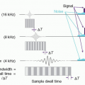
The average acquisition time per reconstructed image slice in a single-slice spin echo sequence is clinically unacceptable. However, the average time per slice is significantly reduced using multislice acquisition methods, where several slices within the tissue volume are selectively excited in a sequential timing scheme during the TR interval to fully utilize the dead time waiting for longitudinal recovery in an adjacent slice, as shown in Figure 13-1. This requires cycling all of the gradients and tuning the RF excitation pulse many times during a single TR interval. The total number of slices that can be acquired simultaneously is a function of TR, TE, and machine limitations:
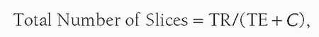
where C is a constant dependent on the MR equipment capabilities (computer speed; gradient capabilities; sequence options; additional pulses, e.g., spoiling pulses in standard SE; use of spatial saturation; and chemical shift, among others). Each slice and each echo, if multiecho, requires its own k-space repository to store data as they are acquired. Long TR acquisitions such as proton density and T2-weighted sequences can produce a greater number of slices over a given volume than T1-weighted sequences with a short TR. The chief trade-off is a loss of tissue contrast due to cross-excitation of adjacent slices due to non-square excitation profiles, causing undesired proton saturation as explained in Section 13.6 on artifacts.
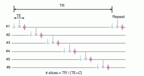 ▪ FIGURE 13-1 Multislice two-dimensional image acquisition is accomplished by discretely exciting different slabs of tissue during the TR period; appropriate changes of the RF excitation bandwidth, SSG, PEG, and FEG parameters are necessary. Because of diffuse excitation profiles, RF irradiation of adjacent slices leads to partial saturation and loss of contrast. The number of slices (volume) that can be obtained is a function of the TR, TE, and C, the latter representing the capabilities of the MR system and type of pulse sequence. |
13.1.3 Acquisition Time, 3D Acquisition
The image acquisition time is equal to
When using a standard TR of 600 ms with one average for a T1-weighted exam, a 128 × 128 × 128 cube requires 163 min or about 2.7 h! Obviously, this is unacceptable for standard clinical imaging. GRE pulse sequences with TR of 50 ms acquire the same image volume in about 15 min. Another shortcut is with anisotropic voxels, where the phase encoding steps in one dimension are reduced, albeit with a loss of resolution.
13.2 FAST IMAGING TECHNIQUES
13.2.1 Fast Pulse Sequences
Fast Spin Echo (FSE) techniques use multiple PEG steps in conjunction with multiple 180° refocusing RF pulses to produce an echo train length (ETL) with corresponding digital data acquisitions per TR interval, as illustrated in Figure 13-2. Multiple k-space rows are filled during each TR equal to the ETL, which is also the reduction factor for acquisition time. “Effective echo time” is determined when the central views in k-space are acquired, which are usually the first echoes, and subsequent echoes are usually spaced apart via increased PEG strength with the same echo spacing time. “Phase re-ordering” optimizes SNR by acquiring the low-frequency information with the early echoes (lowest amount of T2 decay), and the highfrequency, peripheral information with late echoes, where the impact on overall image SNR is lower. The FSE technique has the advantage of spin echo image acquisition, namely immunity from external magnetic field inhomogeneities, with 4×, 8×, to 16× faster acquisition time. However, each echo experiences different amounts of intrinsic T2 decay, which results in image contrast differences and image blurring in
the phase encoding direction when compared with conventional spin echo images of similar TR and TE. Lower signal levels in the later echoes produce less SNR, and fewer images can be acquired in the image volume during the same acquisition. A T2-weighted spin echo image (TR = 2,000 ms, 256 phase encode steps, one average) requires approximately 8.5 min, while a corresponding FSE with an ETL of 4 (Fig. 13-2) requires about 2.1 min. Longer TR values allow for a greater ETL, which will offset the longer TR in terms of overall acquisition time, and will also allow more proton density weighting due to larger Mz recovery. Specific FSE sequences for T2 weighting and multiecho FSE are employed with variations in phase reordering and data acquisition. FSE is also known as “turbo spin echo” or “RARE” (rapid acquisition with refocused echoes).
the phase encoding direction when compared with conventional spin echo images of similar TR and TE. Lower signal levels in the later echoes produce less SNR, and fewer images can be acquired in the image volume during the same acquisition. A T2-weighted spin echo image (TR = 2,000 ms, 256 phase encode steps, one average) requires approximately 8.5 min, while a corresponding FSE with an ETL of 4 (Fig. 13-2) requires about 2.1 min. Longer TR values allow for a greater ETL, which will offset the longer TR in terms of overall acquisition time, and will also allow more proton density weighting due to larger Mz recovery. Specific FSE sequences for T2 weighting and multiecho FSE are employed with variations in phase reordering and data acquisition. FSE is also known as “turbo spin echo” or “RARE” (rapid acquisition with refocused echoes).
 ▪ FIGURE 13-2 Conventional FSE uses multiple 180° refocusing RF pulses per TR interval with incremental changes in the PEG to fill several views in k-space (the ETL). This example illustrates an ETL of four, with an “effective” TE equal to 16 ms. Total time of the acquisition is reduced by the ETL factor. The reversed polarity PEG steps reestablish coherent phase before the next gradient application. Slightly different PEG strengths are applied to fill the center of k-space first, and then the periphery with later echoes, continuing until all views are recorded. As shown, data can be mirrored using conjugate symmetry to reduce the overall time by another factor of two. |
Echo Planar Image (EPI) Acquisition is a technique that provides extremely fast imaging time. Spin Echo (SE-EPI) and Gradient Echo (GRE-EPI) are two methods used for acquiring data, and a third is a hybrid of the two, GRASE (Gradient and Spin Echo). Single-shot (all of the image information is acquired within 1 TR interval) or multishot EPI has been implemented with these methods. For single-shot SE-EPI (Fig. 13-3A), image acquisition typically begins with a standard 90° flip, then a PEG/FEG gradient application to initiate the acquisition of data in the periphery of the
k-space, followed by a 180° echo-producing RF pulse. Immediately after, an oscillating readout gradient and phase encode gradient “blips” are continuously applied to form a gradient echo train and rapidly fill k-space in a stepped “zigzag” pattern. The “effective” echo time occurs at a time TE, when the maximum amplitude of the induced GREs occurs at the center of k-space. Acquisition of the data must proceed in a period less than T2* (around 50 ms), placing high demands on the sampling rate, the gradient coils (shielded coils are required, with low induced “eddy currents”), the RF transmitter/receiver, and RF energy deposition limitations. For GRE-EPI (Fig. 13-3B), a similar acquisition strategy is implemented but without a 180-degree refocusing RF pulse, allowing for faster acquisition time. SE-EPI is generally longer, but better image quality is achieved; on the other hand, larger RF energy deposition to the patient occurs. EPI acquisition can be preceded by any type of RF pulse, for instance FLAIR (EPI-FLAIR), which will produce images much faster than the corresponding conventional FLAIR sequence. EPI acquisitions typically have poor SNR, low resolution (matrices of 64 × 64 or 128 × 64 are typical), and many artifacts, particularly of chemical shift and magnetic susceptibility origin. Nevertheless, EPI offers real-time “snapshot” image capability with 50 ms total acquisition time. EPI is emerging as a clinical tool for studying time-dependent physiologic processes and functional imaging.
Concerns of safety with EPI, chiefly related to the rapid switching of gradients and possible nerve stimulation of the patient, the associated acoustic noise, image artifacts, distortion, and chemical shift are components that limit use for many imaging procedures.
 ▪ FIGURE 13-3 Single shot Echo Planar Spin Echo image (SE-EPI) (A) and Single shot Echo Planar Gradient Recalled Echo image (GRE-EPI) (B) acquisition sequences. Data are deposited in k-space, initially positioned by a simultaneous PEG and FEG application to locate the initial row and column position (in this example, the upper left; for SE-EPI, the 180-degree pulse inverts starting location to upper left), followed by phase encode gradient “blips” simultaneous to FEG oscillations, to fill k-space line by line by introducing 1-row phase changes in a zigzag pattern. Image matrix sizes of 64 × 64 and 128 × 64 are common. |
 ▪ FIGURE 13-4 A Gradient and Spin Echo (GRASE) sequence with three gradient echoes and four fast spin echoes. There are many strategies to efficiently collect 2D or 3D spaces and the example illustrates a case that gradient echoes fill the 3D matrix in the slice direction and spin echoes in the phase encoding direction. Effective TE can be determined by timing the collection of echoes at the center of k-space based on desired image contrast. |
The GRASE (Gradient and Spin Echo) sequence combines the initial spin echo with a series of GREs, followed by an RF rephasing (180°) pulse, and the pattern is repeated until k-space is filled (Fig. 13-4). A GRASE sequence can be utilized for 2D multislice imaging or 3D imaging. The example in the figure describes a 3D imaging application. Although there are variations of terminologies across MRI vendors, general definitions are following: ETL is the number of total echoes acquired in a single TR, an FSE factor is the number of 180° inversion RF pulses inducing spin echoes, and an EPI factor is the number of gradient echoes in a single spin echo. This hybrid sequence achieves the benefits of both types of rephasing: the speed of the gradient and the ability of the RF pulse to compensate for T2* effects, providing significant improvements in image quality compared to the standard EPI methods. A trade-off is a longer acquisition time (e.g., greater than 100 ms) and much greater energy deposition from the multiple 180° RF pulses.
13.2.2 k-Space Filling
Methods to fill k-space in a non-sequential way can increase signal, enhance contrast, and achieve rapid scan times as shown in Figure 13-5. Centric k-space filling has been discussed with FSE imaging (above), where the lower strength phase encode gradients are applied first, filling the center of k-space when the echoes have their highest amplitude. This type of filling is also important for fast GRE techniques, where the image contrast and the SNR fall quickly with time from the initial excitation pulse.
 ▪ FIGURE 13-5 Alternate methods of filling k-space. A. Centric filling applies the lower strength PEGs first to maximize signal and contrast from the earliest echoes of a FSE or GRE sequence. B. Keyhole filling applies PEGs of higher strength first to fill the outer portions of k-space, and the central lines are filled only during a certain part of the sequence, such as with arrival of contrast signal. |
Keyhole filling methods fill k-space similarly to centric filling, except the central lines are filled when important events occur during the sequence, in situations such as contrast-enhanced angiography. Outer areas of k-space are filled first, and when gadolinium appears in the imaging volume, the center areas are filled. At the end of the scan, the outer and central k-space regions are meshed to produce an image with both good contrast and resolution.
13.2.3 Non-Cartesian k-Space Acquisition
The conventional k-space acquisition collects the k-space data in a rectilinear pattern in a Cartesian grid. In some applications, particularly requiring rapid image acquisition, non-Cartesian k-space acquisition schemes have been widely used.
Radial Imaging
Radial imaging was the first method implemented to obtain MR images. However, radial imaging is more susceptible to off-resonance effect and system instabilities, such as field inhomogeneity, eddy-currents, gradient and data acquisition delays, and other effects. k-Space lines can be acquired in a rotating pattern in 2D space (Fig. 13-6A). 3D k-space can be filled with the radial sampling lines with slice encoding steps along z-axis (Fig. 13-6B). Field inhomogeneity, eddy-current, and gradient linearity have been improved in current MR systems. Due to the unique benefit of the tolerance of undersampling, interest in radial imaging has been expanded in volumetric imaging with high undersampling factors such as hybrid projection reconstruction (PR) and 3DPR.
In radial acquisition schemes, all radial spokes pass through the center of a circular k-space and the center has higher sampling density than the periphery. The non-uniform sampling density benefits applications of dynamic (or time-resolved) imaging that requires high temporal resolution, such as contrast-enhanced angiography and cardiac imaging. The redundant information near the center, containing the majority of image contrast, is selected based on the acquisition timing while the sparsely sampled periphery information is shared over different temporal frames, which is called view-sharing. Figure 13-7 describes an example of cardiac imaging using radial acquisitions.
 ▪ FIGURE 13-6 Various non-Cartesian sampling methods: (A) 2D radial sampling with Gx = G0 cos φ and Gy = G0 sin φ. where G0 is the maximum gradient strength, φ is the azimuthal angle of radial line, and full radial lines are acquired with 0 < φ < π. B. 3D radial sampling with Gx = G0 sin θ cos φ, Gy = G0 sin θ sin φ, and Gz = G0 cos θ where θ and φ are the polar angle and the azimuthal angle of radial line, respectively. C. Spiral sampling with sinusoidal oscillation of the x and y gradients 90° out of phase with each other, with samples beginning in the center of k-space and spiraling out to the periphery. |
 ▪ FIGURE 13-7 Illustration of time-resolved cardiac imaging with 2D radial sampling. The radial lines are acquired in an interleaved fashion during one or multiple cardiac cycles. By view sharing, sharing high frequency (periphery of k-space) data with other time frames, the images do not suffer from undersampling artifacts while maintaining the contrast by utilizing full radial lines at a specific time frame. |
Spiral Imaging
Spiral filling is an alternate method of filling k-space radially, which involves the simultaneous oscillation of equivalent encoding gradients to sample data points during echo formation in a spiral, starting at the origin (the center of the k-space) and spiraling outward to the periphery in the prescribed acquisition plane (Fig. 13-6C). The same contrast mechanisms are available in spiral sequences (e.g., T1, T2, proton density weighting), and spin or gradient echoes can be obtained. After acquisition of the signals, an additional postprocessing step, re-gridding, is necessary to convert the spiral data into the rectilinear matrix for two-dimensional Fourier transform (2DFT). Spiral scanning is an efficient method for acquiring data and sampling information in the center of k-space, where the bulk of image information is contained.
Propeller
A variant of radial sampling with enhanced filling of the center of k-space is known generically as “blade” imaging, and commonly as propeller: Periodically Rotated Overlapping Parallel Lines with Enhanced Reconstruction, where a rectangular block of data is acquired and then rotated about the center of k-space. Redundant information concentrated in the center of k-space is used for improvement of SNR or for the identification of times during the scan in which the patient may have moved, so that those blocks of data can be processed with a phase-shifting algorithm to eliminate the movement effect on the data during the reconstruction process and to mitigate motion artifacts to a great extent. Filling of k-space for this method is shown in Figure 13-8.
 ▪ FIGURE 13-8 The propeller data acquisition compared to a rectangular filling of k-space is shown above. Instead of acquiring single lines of information to fill k-space consecutively as shown in the upper left and middle left, a rectangular data acquisition at a specific angle (e.g., 0°) is acquired encompassing several lines of k-space, which represents a “blade” of information. The partial acquisition is rotated about the center of k-space at angular increments, which provides a dense sampling of data at the center of k-space and less in the periphery as shown by the schematic (upper right illustration). If the patient moves during a portion of the examination (lower left image), the blades in which the motion occurred can be identified and reprocessed, and the image reconstructed without the motion artifacts (lower right image). |
13.2.4 Data Synthesis
Data “synthesis” takes advantage of the symmetry and redundant characteristics of the frequency domain signals in k-space. The acquisition of as little as one half the data plus one row of k-space allows the mirroring of “complex conjugate” data to fill the remainder of the matrix (Fig. 13-9). In the phase encode direction, “half Fourier,” “½ NEX,” or “phase conjugate symmetry” (vendor-specific naming) techniques effectively reduce the number of required TR intervals by one half plus one line, and thus can reduce the acquisition time by nearly one half. In the frequency encoding direction, “fractional echo” or “read conjugate symmetry” refers to reading a fraction of the echo. While there is no scan time reduction when all the phase encode steps are acquired, there is a significant echo time reduction, which allows more slices to be covered in one TR or reduces motion-related artifacts, such as dephasing of blood. However, the penalty for either half Fourier or fractional echo techniques is a reduction in the SNR (caused by a reduced NEX or data sampling in the volume). If the approximations in the complex conjugation of the signals are not accurate mainly due to the factors causing phase incoherence of spins, artifacts may present and collecting k-space by more than a half (i.e., 5/8 NEX) is desired. The factors yielding phase incoherence include inhomogeneities of the magnetic field, imperfect linear gradient fields, and the presence of magnetic susceptibility agents in the volume being imaged.
 ▪ FIGURE 13-9 Fractional NEX and fractional echo. Left: Data synthesis uses the redundant characteristics of the frequency domain. This is an example of phase conjugate symmetry, in which ½ of the PEG views +1 extra are acquired, and the complex conjugate of the data is reflected in the symmetric quadrants. Acquisition time is thus reduced by approximately 2× (˜50%) although image noise is increased by approximately  (40%). Right: Fractional echo acquisition is performed when only part of the echo is read during the application of the FEG. Usually, the peak of the echo is centered in the middle of the readout gradient, and the echo signals prior to the peak are identical mirror images after the peak. With fractional echo, the echo is no longer centered, and the sampling window is shifted such that only the peak echo and the dephasing part of the echo are sampled. As the peak of the echo is closer to the RF excitation pulse, TE can be reduced, which can improve T1 and proton density weighting contrast. A larger number of slices can also be obtained with a shorter TE in a multislice acquisition (see Fig. 13-2). (40%). Right: Fractional echo acquisition is performed when only part of the echo is read during the application of the FEG. Usually, the peak of the echo is centered in the middle of the readout gradient, and the echo signals prior to the peak are identical mirror images after the peak. With fractional echo, the echo is no longer centered, and the sampling window is shifted such that only the peak echo and the dephasing part of the echo are sampled. As the peak of the echo is closer to the RF excitation pulse, TE can be reduced, which can improve T1 and proton density weighting contrast. A larger number of slices can also be obtained with a shorter TE in a multislice acquisition (see Fig. 13-2). |
13.2.5 Parallel Imaging
Acquiring k-space information quickly is desired in many applications in order to reduce motion artifact as well as a scan time. Without compromise of image resolution, only a part of k-space can be acquired as shown in Figure 13-10A. However, because the field of view (FOV) dimension in the phase encode direction is inversely proportional to the spacing, the size of the effective FOV is reduced to 1/N its original size, and as a result, aliasing of signals outside of the FOV in the phase encode direction occurs.
Parallel imaging is a technique that overcomes the aliasing artifacts due to undersampling by using the response of multiple receive RF coils that are coupled together with independent channels, so that data can be acquired simultaneously. Specific hardware and software are necessary for the electronic orchestration of this capability. Typically, 2, 4, 8, 16, 24 (or more) coils are arranged around the area to be imaged; if a 4-coil configuration is used, then during each TR period, each coil acquires a view of the data as the acquisition sequence proceeds. Lines in k-space are defined only after the processing of linear combinations of the signals that are received by all of the coils. If 4 views of the data are acquired per TR interval, in the ideal situation, scan time can be decreased by a factor of 4 (known as the reduction factor or acceleration factor). One of the approaches, called SENSitivity Encoding (SENSE),
uses the sensitivity profile of each coil to calculate where the signal is coming from relative to the coil based on its amplitude—the signal generated near the coil has a higher amplitude than the signal furthest away. Depending on the geometrical configuration of coils, an individual coil may have unique spatial information that other coils do not have. The unwrapped images can be expressed as a linear combination of acquired images from each coil times the coil sensitivity of each coil (Fig. 13-10B). With knowledge of the coil sensitivities, the unwrapped images can be generated by solving a linear equation per voxel. The coil sensitivity can be measured by a short separate calibration scan prior to the undersampling scan or by generating low resolution images from the image itself by acquiring additional lines near the center of k-space (referred to as self-calibration).
uses the sensitivity profile of each coil to calculate where the signal is coming from relative to the coil based on its amplitude—the signal generated near the coil has a higher amplitude than the signal furthest away. Depending on the geometrical configuration of coils, an individual coil may have unique spatial information that other coils do not have. The unwrapped images can be expressed as a linear combination of acquired images from each coil times the coil sensitivity of each coil (Fig. 13-10B). With knowledge of the coil sensitivities, the unwrapped images can be generated by solving a linear equation per voxel. The coil sensitivity can be measured by a short separate calibration scan prior to the undersampling scan or by generating low resolution images from the image itself by acquiring additional lines near the center of k-space (referred to as self-calibration).
Parallel imaging can also be achieved by synthesizing the skipped k-space lines directly and generating unwrapped images from an individual coil. Coil sensitivity in image space corresponds to a convolution kernel in k-space (a multiplication in image space is equivalent to a convolution in frequency space). The convolution operation is essentially a linear operation of neighboring voxels, and the redundant information from multiple coil elements allows synthesizing the missing information as shown in Figure 13-10C. After the missing k-space lines are filled up, images from each coil are generated and combined to create the final images. Similar to coil sensitivity measurement, the convolution kernel of each coil can be estimated by acquiring additional
lines near the center of k-space and a representative method is GeneRalized Autocalibrating Partially Parallel Acquisition (GRAPPA).
lines near the center of k-space and a representative method is GeneRalized Autocalibrating Partially Parallel Acquisition (GRAPPA).
 ▪ FIGURE 13-10 Image reconstruction with undersampled k-space by acquiring a half of data (every odd line): (A) Conventional reconstruction showed imaging aliasing (wrap-around) because the size of the effective FOV is reduced to a half of its original size. B. Image based sensitivity encoding utilizes the sensitivity profile of each coil to calculate where the signal is coming from relative to the coil based on its amplitude. With a priori knowledge of the coil sensitivities, the unwrapped images can be generated by solving a linear equation per voxel. C. k-space based methods synthesize the skipped k-space lines directly and generate unwrapped images from an individual coil using coil specific convolution kernels estimated by auto-calibration. |
Parallel imaging can be used to either reduce scan time or improve resolution, in conjunction with most pulse sequences. In addition, it significantly reduces geometric distortion present in EPI. Downsides include image misalignment between a calibration scan and an actual scan due to patient motion and, more importantly, an SNR penalty. The SNR of parallel imaging is

where SNRFully Sampled is the SNR of fully sampled image, R is the scan time reduction factor, and g is the coil geometry factor. Although the example shown in Figure 13-10 has ideal coil sensitivities with sharp boundaries, the actual coil sensitivity is reduced as further apart from each coil location. Therefore, a part of image volume (usually the center) is detectable by multiple coil elements and the geometry factor, g-factor, is determined by the number of aliased replications on each voxel that varies by location across the image.
As the example shows, the acceleration is done in the phase encoding direction in 2D imaging; however, the acceleration can be done in either phase encoding or slice encoding directions in 3D imaging. Considering the direction of acceleration, the coil geometry should be reviewed. Choosing the acceleration direction into the direction that has the most coil elements guarantees the best performance in terms of SNR and residual aliasing artifacts. For example, if the parallel imaging direction is chosen in the A/P direction during a spine exam with a spine coil, parallel imaging will not be performed correctly and images will have severe aliasing artifacts.
13.2.6 Multiband Imaging
Multiband (MB) imaging (or simultaneous multislice [SMS]) is a technique to further accelerate image acquisition, primarily for 2D multislice imaging. Recent advances in parallel imaging enable unwrapping the aliased image in the slice direction when multiple slices are excited and acquired simultaneously. Figure 13-11 describes a simple example of MB imaging with an MB factor of 2, meaning two slices are excited together. In 2D axial acquisition, multiple slices can be excited by a single RF pulse that has two distinct resonance frequencies or two sequential RF pulses that each has a unique resonance frequency. When multiple slices are excited, the FOV of slices are shifted by a factor of FOV/MB in order to minimize the overlapped area and improve the g-factor in the reconstruction. For example, when two slices are excited, one of the slices that locates off the gradient isocenter is shifted by FOV/2 as shown in the figure. This is done by adding a small gradient in the z-direction. The acquired image with MB excitation shows multiple slices together, and the unwrapping is done by a parallel imaging technique applied in the slice encoding direction. Although the actual acquisition is done in 2D image space, the image reconstruction handles the data as 3D imaging. While parallel imaging has an SNR penalty because of reduced phase (or slice) encoding lines, MB imaging does not have this penalty and only the coil g-factor in the slice direction affects SNR. This SNR advantage allows high MB factors if a coil has very high number of channels, such as 32 or 64 channels. Thus, the MB imaging is often utilized in conjunction with parallel imaging for further acceleration. For example, an acceleration factor of 8 (MB factor of 4 × parallel imaging factor of 2) or higher is feasible without much SNR loss or artifacts.
 ▪ FIGURE 13-11 Multiband imaging excites multiple slices simultaneously and unwraps the aliased image in the slice direction using a parallel imaging approach. There is no SNR penalty besides the coil geometry factor because a larger signal is received with multiple 2D slices. This enables a high acceleration factor along with parallel imaging. |
13.3 SIGNAL FROM FLOW
The appearance of moving fluid (vascular and cerebrospinal fluid [CSF]) in MR images is complicated by many factors, including flow velocity, vessel orientation, laminar versus turbulent flow patterns, pulse sequences, and image acquisition modes. Flow-related mechanisms combine with image acquisition parameters to alter contrast. Signal due to flow covers the entire gray scale of MR signal intensities, from “black blood” to “bright blood” levels, and flow can be a source of artifacts. The signal from flow can also be exploited to produce MR angiographic images.
Low signal intensities (flow voids) are often a result of high-velocity signal loss (HVSL), in which protons in the flowing blood move out of the slice during echo reformation, causing a lower signal. Flow turbulence can also cause flow voids, by causing a dephasing of protons in the blood with a resulting loss of the tissue magnetization in the area of turbulence. With HVSL, the amount of signal loss depends on the velocity of the moving fluid. Pulse sequences to produce “black blood” in images can be very useful in cardiac and vascular imaging. A typical black blood pulse sequence uses a “double inversion recovery” method, whereby a non-selective 180° RF pulse is initially applied, inverting all protons in the active volume, and is followed by a selective 180° RF pulse that restores the magnetization in the selected slice. During the inversion time, blood with inverted protons outside of the excited slice flows into the slice, producing no signal; therefore, the blood appears dark.
13.3.1 Flow-Related Enhancement
Flow-related enhancement is a process that causes increased signal intensity due to flowing protons; it occurs during imaging of a volume of tissues. Flow enhancement in GRE images is pronounced for both venous and arterial structures, as well as CSF. The high intensity is caused by the wash-in (between subsequent RF excitations) of fully unsaturated protons into a volume of partially saturated protons due to the
short TR used with gradient imaging. During the next excitation, the signal amplitude resulting from the moving unsaturated protons is about 10 times greater than that of the non-moving saturated protons. With GRE techniques, the degree of enhancement depends on the velocity of the blood, the slice or volume thickness, and the TR. As blood velocity increases, unsaturated blood exhibits the greatest signal. Similarly, a thinner slice or decreased repetition time results in higher flow enhancement. In arterial imaging of high-velocity flow, it is possible to have bright blood throughout the imaging volume of a three-dimensional acquisition if unsaturated blood can penetrate into the volume prior to experiencing an RF pulse.
short TR used with gradient imaging. During the next excitation, the signal amplitude resulting from the moving unsaturated protons is about 10 times greater than that of the non-moving saturated protons. With GRE techniques, the degree of enhancement depends on the velocity of the blood, the slice or volume thickness, and the TR. As blood velocity increases, unsaturated blood exhibits the greatest signal. Similarly, a thinner slice or decreased repetition time results in higher flow enhancement. In arterial imaging of high-velocity flow, it is possible to have bright blood throughout the imaging volume of a three-dimensional acquisition if unsaturated blood can penetrate into the volume prior to experiencing an RF pulse.
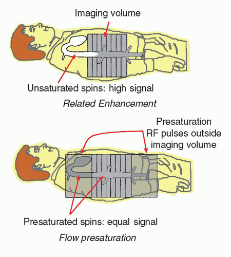 ▪ FIGURE 13-12 The repeated RF excitation within an imaging volume produces partial saturation of the tissue magnetization (top figure, gray area). Unsaturated protons flowing into the volume generate a large signal difference that is bright relative to the surrounding tissues. Bright blood effects can be reduced by applying presaturation RF pulses adjacent to the imaging volume, so that protons in inflowing blood will have a similar partial saturation (bottom figure; note no blood signal). |
Signal from blood is dependent on the relative saturation of the surrounding tissues and the incoming blood flow in the vasculature. In a multislice volume, repeated excitation of the tissues and blood causes a partial saturation of the protons, dependent on the T1 characteristics and the TR of the pulse sequence. Blood outside of the imaged volume does not interact with the RF excitations, and therefore these unsaturated protons may enter the imaged volume and produce a large signal compared to the blood within the volume. This is known as flow-related enhancement. As the pulse sequence continues, the unsaturated blood becomes partially saturated and the protons of the blood produce a similar signal to the tissues in the inner slices of the volume (Fig. 13-12). In some situations, flow-related enhancement is undesirable and is eliminated with the use of “presaturation” pulses applied to volumes just above and below the imaging volume. These same saturation pulses are also helpful in reducing motion artifacts caused by adjacent tissues outside the imaging volume.
13.3.2 MR Angiography
Exploitation of blood flow enhancement is the basis for MRA. Two techniques to create images of vascular anatomy include time-of-flight and phase contrast angiography.
Time-of-Flight Angiography
The time-of-flight technique relies on the tagging of blood in one region of the body and detecting it in another. This differentiates moving blood from the surround ing stationary tissues. Tagging is accomplished by proton saturation, inversion, or
relaxation to change the longitudinal magnetization of moving blood. The penetration of the tagged blood into a volume depends on the T1, velocity, and direction of the blood. Since the detectable range is limited by the eventual saturation of the tagged blood, long vessels are difficult to visualize simultaneously in a threedimensional volume. For these reasons, a two-dimensional stack of slices is typically acquired, where even slowly moving blood can penetrate the region of RF excitation in thin slices (Fig. 13-13). Each slice is acquired separately, and blood moving in one direction (north or south, e.g., arteries versus veins) can be selected by delivering a presaturation pulse on an adjacent slab superior or inferior to the slab of data acquisition. Thin slices are also helpful in preserving resolution of the flow pattern. Often used for the two-dimensional image acquisition is a “GRASS” or “FISP” GRE technique that produces relatively poor anatomic contrast yet provides a high-contrast “bright blood” signal. Magnetization transfer contrast sequences (see below) are also employed to increase the contrast of the signals due to blood by reducing the background anatomic contrast.
relaxation to change the longitudinal magnetization of moving blood. The penetration of the tagged blood into a volume depends on the T1, velocity, and direction of the blood. Since the detectable range is limited by the eventual saturation of the tagged blood, long vessels are difficult to visualize simultaneously in a threedimensional volume. For these reasons, a two-dimensional stack of slices is typically acquired, where even slowly moving blood can penetrate the region of RF excitation in thin slices (Fig. 13-13). Each slice is acquired separately, and blood moving in one direction (north or south, e.g., arteries versus veins) can be selected by delivering a presaturation pulse on an adjacent slab superior or inferior to the slab of data acquisition. Thin slices are also helpful in preserving resolution of the flow pattern. Often used for the two-dimensional image acquisition is a “GRASS” or “FISP” GRE technique that produces relatively poor anatomic contrast yet provides a high-contrast “bright blood” signal. Magnetization transfer contrast sequences (see below) are also employed to increase the contrast of the signals due to blood by reducing the background anatomic contrast.
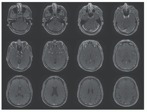 ▪ FIGURE 13-13 The time of flight MRA acquisition collects each slice separately with a sequence to enhance blood flow. Exploitation of blood flow is achieved by detecting unsaturated protons moving into the volume, producing a bright signal. A coherent GRE image acquisition pulse sequence is shown, TR = 24 ms, TE = 3.1 ms, flip angle = 20°. Every 10th image in the stack is displayed above, from left to right and top to bottom. |
Two-dimensional TOF MRA images are obtained by projecting the content of the stack of slices at a specific angle through the volume. A maximum intensity projection (MIP) algorithm detects the largest signal along a given ray through the volume and places this value in the image (Fig. 13-14). The superimposition of residual stationary anatomy often requires further data manipulation to suppress undesirable signals. This is achieved in a variety of ways, the simplest of which is setting a window threshold. Another method is to acquire a dataset without contrast and subtract the non-contrast MIP from the contrast MIP to reduce background signals. Clinical MRA images show the three-dimensional characteristics of the vascular anatomy from several angles around the volume stack (Fig. 13-15) with some residual signals from the stationary anatomy. Time-of-flight angiography often produces variation in vessel intensity dependent on orientation with respect to the image plane, a situation that is less than optimal.
 ▪ FIGURE 13-14 A simple illustration shows how the MIP algorithm extracts the highest (maximum) signals in the two-dimensional stack of images along a specific direction in the volume, and produces projection images with maximum intensity variations as a function of angle. |
Phase Contrast Angiography
Phase contrast imaging relies on the phase change that occurs in moving protons such as blood. One method of inducing a phase change is dependent on the application of a bipolar gradient in the direction of the bipolar gradients (one gradient with positive polarity followed by a second gradient with negative polarity, separated by a delay time ΔT). There are many factors other than flow that causes a phase offset, such as off-resonance fields, chemical shift, motion, and temperature. To remove this phase offset, another image is acquired with opposite gradients. In a second acquisition of the same view of the data (same PEG), the polarity of the bipolar gradients is reversed, and moving protons show phases in the opposite direction, while the
stationary protons exhibit no phase differences (Fig. 13-16). Subtracting the phase of the second excitation from the first cancels the phase of stationary protons but doubles the phase of moving protons. Alternating the bipolar gradient polarity for each subsequent excitation during the acquisition provides phase contrast image information. The degree of phase shift is directly related to the velocity encoding (VENC) time, ΔT, between the positive and negative lobes of the bipolar gradients, the area of velocity encoding gradients, and the velocity of the protons within the excited volume. Proper selection of the VENC time and gradient areas is necessary to avoid phase wrap error (exceeding 180° phase differences) and to ensure an optimal phase shift range for the velocities encountered. In the phase image, intensity variations are dependent on the amount of phase shift, where the brightest pixel values represent the largest forward (or backward) velocity, a mid-scale value represents 0 velocity, and the darkest pixel values represent the largest backward (or forward) velocity. Figure 13-17 shows a representative magnitude and phase contrast image of the cardiac vasculature. Unlike the time-of-flight methods, the phase contrast image is inherently quantitative and, when calibrated carefully, provides an estimate of the mean blood flow velocity and direction. Two- and three-dimensional phase contrast image acquisitions for MRA are possible.
stationary protons exhibit no phase differences (Fig. 13-16). Subtracting the phase of the second excitation from the first cancels the phase of stationary protons but doubles the phase of moving protons. Alternating the bipolar gradient polarity for each subsequent excitation during the acquisition provides phase contrast image information. The degree of phase shift is directly related to the velocity encoding (VENC) time, ΔT, between the positive and negative lobes of the bipolar gradients, the area of velocity encoding gradients, and the velocity of the protons within the excited volume. Proper selection of the VENC time and gradient areas is necessary to avoid phase wrap error (exceeding 180° phase differences) and to ensure an optimal phase shift range for the velocities encountered. In the phase image, intensity variations are dependent on the amount of phase shift, where the brightest pixel values represent the largest forward (or backward) velocity, a mid-scale value represents 0 velocity, and the darkest pixel values represent the largest backward (or forward) velocity. Figure 13-17 shows a representative magnitude and phase contrast image of the cardiac vasculature. Unlike the time-of-flight methods, the phase contrast image is inherently quantitative and, when calibrated carefully, provides an estimate of the mean blood flow velocity and direction. Two- and three-dimensional phase contrast image acquisitions for MRA are possible.
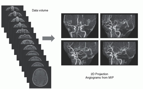 ▪ FIGURE 13-15 A volume stack of bright blood images (left) is used with MIP processing to create a series of projection angiograms at regular intervals; the three-dimensional perspective is appreciated in a stack view, with virtual rotation of the vasculature. |
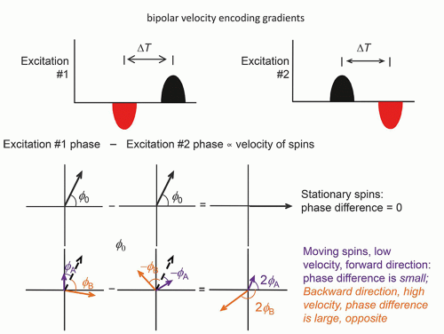 ▪ FIGURE 13-16 Phase contrast angiography uses consecutive excitations that have a bipolar gradient encoding with the polarity reversed between the first and second excitation, as shown in the top row. Magnetization vectors (lower two rows) illustrate the effect of the bipolar gradients on stationary and moving spins for the first and second excitations. Subtracting the phases of two spins will cancel stationary tissue phase and enhance phase differences caused by the velocity of moving blood. |
13.3.3 Gradient Moment Nulling
In spin echo or gradient recalled echo imaging, the slice select and readout gradients are balanced, so that the uniform dephasing with the initial gradient application
is rephased by an opposite polarity gradient of equal area. However, when moving protons are subjected to the gradients, the amount of phase dispersion is not compensated (Fig. 13-18). This phase dispersal can cause ghosting (faint, displaced copies of the anatomy) in images. It is possible, however, to rephase the protons by a gradient moment nulling technique. With constant velocity flow (first-order motion), all protons can be rephased using the application of a gradient triplet. In this technique, an initial positive gradient of unit area is followed by a negative gradient of twice the area, which creates phase changes that are compensated by a third positive gradient of unit area. The velocity compensated gradient (right graph in Fig. 13-18) depicts the evolution of the proton phase back to zero for both stationary and moving protons. Note that the overall applied gradient has a net area of zero—equal to the sum of the positive and negative areas. Higher order corrections such as second- or
third-order moment nulling to correct for acceleration and other motions are possible, but these techniques require more complicated gradient switching. Gradient moment nulling can be applied to both the slice select and readout gradients to correct for problems such as motion ghosting as elicited by CSF pulsatile flow. This approach is also referred to as flow-compensation.
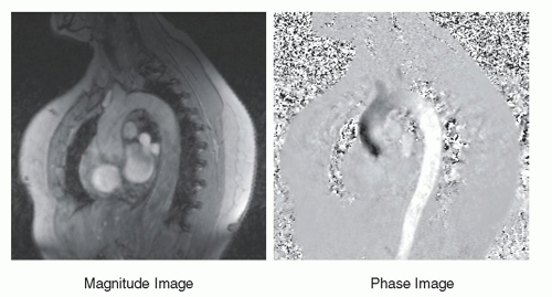 ▪ FIGURE 13-17 Magnitude (left) and phase (right) images provide contrast of flowing blood. Magnitude images are sensitive to flow, but not to direction; phase images provide direction and velocity information. The blood flow from the heart shows forward flow in the ascending aorta (dark area) and forward flow in the descending aorta at this point in the heart cycle for the phase image. Some bright flow patterns in the ascending aorta represent backward flow to the coronary arteries. Grayscale amplitude is proportional to velocity, where intermediate grayscale is 0 velocity. |
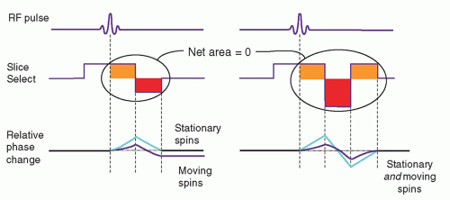 ▪ FIGURE 13-18 Left: Phase dispersion of stationary and moving spins under the influence of an applied gradient (no flow compensation) as the gradient is inverted is shown. The stationary spins return to the original phase state, whereas the moving spins do not. Right: Gradient moment nulling of first order linear velocity (flow compensation) requires a doubling of the negative gradient amplitude followed by a positive gradient such that the total summed area is equal to zero. This will return both the stationary spins and the moving spins to their original phase state. |
13.4 PERFUSION AND DIFFUSION CONTRAST IMAGING
Perfusion is the delivery of blood to a capillary bed in tissue and permits the delivery of oxygen and nutrients to the cells and removal of waste (e.g., CO2) from the cells. There are many perfusion parameters that are estimated using MRI. Blood flow is the rate at which blood is delivered to tissues. Blood volume is the fraction of blood volume in tissues. Mean transit time (MTT) is the average time during which a tracer resides within the system. Lastly, vessel permeability is the transfer of a tracer from intravascular space to extravascular-extracellular space. These parameters are related to the vascular physiology. Hyper or hypo metabolism or ischemia is reflected to the amount of blood flow. Abnormal vascularization such as angiogenesis of tumor or stenosis affects blood volume and MTT. In the brain, when the blood-brain barrier (BBB) is broken down, vessel permeability is also changed. Conventional perfusion measurements are based on the uptake and wash-out of radioactive tracers or other exogenous tracers that can be quantified from image sequences using well-characterized imaging equipment and calibration procedures. For MR perfusion images, exogenous and endogenous tracer methods are used. As an endogenous contrast, blood itself can be a contrast tracer because blood is freely diffusible into tissue including the interior of cells. Arterial spin labeling (ASL) technique uses the blood magnetization. Another approach uses Gadolinium (Gd) based contrast agent. Gd is a paramagnetic element that shortens T2/T2* and T1 of surrounding tissue. Most of the Gd based contrast agent is an extracellular tracer that passes through vessel walls, but not in the brain because of the blood-brain barrier. Dynamic susceptibility contrast (DSC) MRI and dynamic contrast enhanced (DCE) MRI are in this category.
13.4.1 Arterial Spin Labeling
ASL technique uses the blood magnetization and measures blood flow. There are two popular ASL techniques based on a blood tagging scheme (Fig. 13-19). One is pulsed ASL and the other is continuous ASL. In pulsed ASL, a 180° RF pulse inverts the blood signal in the neck, and a 90° saturation pulse is applied later to the same location in order to convert the spatial bolus into temporal bolus. After a 1-2 s waiting time for blood to be delivered to the tissue, images in the target region are obtained. Another set of images without blood inversion is acquired (called control) and subtracted from the images in which blood signals are inverted. The subtraction removes signals from static tissues. For continuous or pseudo-continuous ASL, a long RF pulse or a train of RF pulses is applied in the neck while the blood signal passing through the plane is inverted. After waiting time for blood to be delivered to the tissue (often called postlabeling delay), images in the target region are acquired. Same as pulsed ASL, another set of images is collected while blood signals are non-inverted and subtracted from the tagged images. The signals are derived from blood signals, which are a small fraction (1%-2%) of brain or tissue, so ASL imaging suffers from low SNR. 2D imaging needs multiple signal averages (20-60) to overcome the low SNR. 3D imaging, which provides higher SNR, is often preferred but is sensitive to motion. Background suppression is often applied with multiple inversion pulses in order to
reduce static signals, such as gray and white matter, and improve SNR of ASL images. The most important issue in ASL imaging is choice of the waiting time. If the images are acquired too early, the signals observed in image are only vascular signals, not true tissue perfusion. In case of a sufficiently long waiting time, only tissue perfusion signals are measured, but the SNR is decreased because of T1 decay of blood signals.
reduce static signals, such as gray and white matter, and improve SNR of ASL images. The most important issue in ASL imaging is choice of the waiting time. If the images are acquired too early, the signals observed in image are only vascular signals, not true tissue perfusion. In case of a sufficiently long waiting time, only tissue perfusion signals are measured, but the SNR is decreased because of T1 decay of blood signals.
Related posts:
 X-ray Production, Tubes, and Generators
 X-ray Dosimetry in Projection Imaging and Computed Tomography
 Radiation Detection and Measurement
 Magnetic Resonance Basics: Magnetic Fields, Nuclear Magnetic Characteristics, Tissue Contrast, Image Acquisition
Stay updated, free articles. Join our Telegram channel

Full access? Get Clinical Tree


