Medicine Dose Assessment

(1)

where $\mathop D\limits^{ \bullet }_{T}$ = absorbed dose rate to a target region of interest (Gy/sec or rad/hr)

A _S = activity (MBq or μCi) in source region S

y _i = number of radiations with energy E _iemitted per nuclear transition

E _i = energy per radiation for the ith radiation (MeV)

ϕ_i = fraction of energy emitted n a source region that is absorbed in a target region

m _T = mass of the target region (kg or g)

k = proportionality constant (Gy-kg/MBq-sec-MeV or rad-g/μCi-hr-MeV).

The proportionality constant k includes the various factors that are needed to obtain the dose rate in the desired units, from the units employed for the other variables, and it is essential that this factor is properly calculated and applied. For example, if we want the dose rate in rad/hr, and we have employed units of μCi for activity, MeV for energy, and g for mass, the conversions that are needed are:

$k = \frac{{3.7\, \times \,10^{4} \;{\text{dis}}}}{\sec - \mu Ci}\frac{3600\;\sec }{\text{hr}}\frac{{{\text{rad}} - g}}{{100\;{\text{erg}}}}\frac{{1.6\, \times \,10^{ - 6} \;{\text{erg}}}}{{1\;{\text{MeV}}}} = 2.13\;\frac{{{\text{rad}} - g}}{{\mu Ci - {\text{hr}} - {\text{MeV}}}}$

If instead we want the dose rate in Gy/sec, and we have employed units of MBq for activity, MeV for energy, and kg for mass, the conversions that are needed are:

$k = \frac{{1\;{\text{dis}}}}{{\sec - {\text{MBq}}}}\frac{{{\text{Gy}} - {\text{kg}}}}{1\;J}\frac{{1.6 \times 10^{ - 13} \;J/{\text MeV}}}{{1\;{\text{MeV}}}}\frac{{1000\;{\text{mGy}}}}{\text{Gy}} = 1.6\, \times \,10^{ - 10} \;\frac{{{\text{mGy}} - {\text{kg}}}}{{{\text{MBq}} - {\text s} - {\text{MeV}}}}$

Most calculations are based on total absorbed dose, rather than just the dose rate at some point in time. In the dose equation above, the quantity activity (nuclear transitions per unit time) causes the outcome of the equation to have a time dependence. To calculate cumulative dose, the time integral of the dose equation must be calculated. In most cases, the only term which depends on time is activity, so the only factor that has to be integrated is the activity term. The integral of the time-activity curve (i.e., the area under that curve, regardless of its shape), is often called the cumulated activity (often given with the symbol Ã), and it represents the total number of disintegrations that have occurred over time in a source region (Fig. 1).

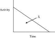
Fig. 1

General time/activity curve for an internal emitter

Therefore, the equation for cumulative dose becomes:

$D_{T} = \int {\mathop {D_{T} }\limits^{ \bullet } \;{\text{d}}t} = \frac{{k\;\mathop {A_{S} }\limits^{\sim } \sum\limits_{i} {y_{i} \;E_{i} \;\phi_{i} } }}{{m_{T} }}$

(2)

where D is the absorbed dose (Gy or rad), and the quantity Ã _Srepresents the integral of A _S(t), the time-dependent activity within the source region:

$\mathop {\tilde{A}_{S}} = \int\limits_{0}^{\infty } {\mathop {\tilde{A}_{S}} (t)\;{\text{d}}t = } A_{0} \int\limits_{0}^{\infty } {f_{S} (t)\;{\text{d}}t}$

(3)

where A ₀is the activity administered to the patient at time t = 0, and f _S(t) may be called the fractional distribution function for a source region (fraction of administered activity present within the source region at time t). In many instances, the function f _S(t) may be modeled as a sum of exponential functions:

$f_{S} (t) = f_{1} \;e^{{ - (\lambda_{i} + \lambda_{p} )t}} + f_{2} \;e^{{ - (\lambda_{2} + \lambda_{p} )t}} + \cdots + f_{N} \;e^{{ - (\lambda_{N} + \lambda_{p} )t}}$

(4)

where terms f ₁…f _Nrepresent the fractional uptake of the administered activity within the 1st to Nth compartments of the source region, λ ₁…λ _Nrepresent the biological elimination constants for these same compartments, and λ _Prepresents the physical decay constant for the radionuclide of interest. Other functional expressions may be used to represent the fractional distribution function, but exponentials are most commonly encountered.

A generalized expression for calculating internal dose, which may describe the equations shown in publications by different authors, can be calculated by the following equation:

$D = N \times {\text{DF}}$

(5)

where N is the number of nuclear transitions that occur in source region S (identical to Ã _S), and DF is a “dose factor”. The factor DF contains the various components shown in the formulas for S and SEE; basically it depends on combining decay data with absorbed fractions (AFs), which are derived generally using Monte Carlo simulation of radiation transport in models of the body and its internal structures (organs, tumors, etc.):

${\text{DF}} = \frac{{k\sum\limits_{i} {y_{i} \;E_{i} \;\phi_{i} \;w_{{R_{i} }} } }}{{m_{T} }}$

(6)

As written, the above equations give only the dose from one source region to one target region, but they can be generalized easily to multiple source regions:

$D_{T} = \frac{{k\sum\limits_{S} {\mathop {A_{S} }\limits^{\sim } } \;\sum\limits_{i} {y_{i} \;E_{i} \;\phi_{i} (T \leftarrow S)} \;w_{{R_{i} }} }}{{m_{T} }}$

(7)

An important exception to the statement above that activity is the only term in the dose equation that varies with time is the need to account for the change in thyroid mass during therapy for hyperthyroidism with ¹³¹I-NaI, as demonstrated by Traino et al. (2000) They recommended a prescribed activity for each subject’s therapy as:

$A_{0} = - \frac{{2\;\ln (2)\;m_{0} }}{{\Updelta_{np} \;\alpha \;[\ln (2)\;T_{\max } + 2\;T_{eff} }}\ln \frac{{m_{fin} }}{{m_{0} }}$

(8)

where m ₀ is the initial thyroid mass, m _fin is the final thyroid mass (measured by ultrasound), Δ_np is the sum of the k × y _i × E _iterms in the dose equation for “nonpenetrating” emissions (principally beta particles in this case), α is a rate constant for the decrease in thyroid mass over time, and T _max and T _eff are the times of maximum thyroid uptake and effective half-time for removal of thyroid activity. These authors found that not performing a patient-specific evaluation of thyroid uptake and the change in mass over time resulted in a 9–30 % difference in the estimate of thyroid dose in these treatments.

3.2 Dose Calculations Based on Animal Data

Preclinical data are needed to begin the approval process for new therapeutic pharmaceuticals. Data collected regarding the activity concentrations in the animal organs may be reasonably extrapolated to humans using the % kg/g method (Kirschner et al. 1975). In this method, the animal organ data need to be reported as % of injected activity per gram of tissue, and this information plus knowledge of the animal whole body weight are employed in the following extrapolation:

$\left( {\frac{\% }{\text{organ}}} \right)_{\text{human}} = \left[ {\left( {\frac{\% }{{g_{\text{organ}} }}} \right)_{\text{animal}} x(kg_{\text{TBweight}} )_{\text{animal}} } \right]x\left( {\frac{{g_{\text{organ}} }}{{kg_{\text{TBweight}} }}} \right)_{\text{human}}$

(9)

For therapeutic radionuclides, it may also be of interest to calculate dose to the organs of the animals. A number of investigators have developed individual rodent models for use in dose calculations (e.g. (Hui et al. 1994; Yoriyaz and Stabin 1997; Muthuswamy et al. 1998; Flynn et al. 2001; Konijnenberg et al. 2004; Hindorf et al. 2004; Kolbert et al. 2003; Stabin et al. 2006). A series of three mouse and five rat models based on the realistic modeling approach of Segars and Tsui (2007) were developed by Keenan et al. (Keenan et al. 2010). Figure 2 shows images of the unmodified rat (ROBY) and mouse (MOBY) models that were scaled to create larger and smaller models, to provide a series of models for use in internal or external dose calculations.

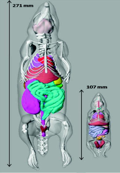
Fig. 2

Images of the unmodified ROBY and MOBY models, showing the length of each model

3.2.1 Examples

In his textbook on nuclear medicine dosimetry, Stabin (2008) provided the following example calculation of data extrapolated from an animal species to the human using the Kirschner et al. approach (Kirschner et al. 1975):

Assuming an animal whole body mass of 20 g (0.02 kg), and a human source organ mass of 300 g, and a human total body mass of 70 kg, the values in the bottom row of the table are calculated from those in the animal %/g row, for example (Table 1):

Table 1

Animal data extrapolation example (Mass extrapolation)

	Source organ
Animal	1 h	3 h	6 h	16 h	24 h
%/Organ	3.79	3.55	2.82	1.02	0.585
(%/g)	38.1	36.6	30.8	11.3	5.70
Human
%/Organ	3.26	3.12	2.63	0.962	0.486

$\frac{38.1\;\% }{\text{g}}\;({\text{animal}}) \times 0.020\;{\text{kg}} \times \frac{{299\;{\text{g}}}}{{70\;{\text{kg}}}} = \frac{3.26\;\% }{\text{organ}}\;({\text{human}})$

One may also perform a transformation of the timescale, to account for the differences in metabolic rate among species of different body mass, which some have suggested can affect the rates at which substances are cleared from the body. One suggested scaling approach is given as:

$t_{h} = t_{a} \left[ {\frac{{m_{h} }}{{m_{a} }}} \right]^{0.25}$

(10)

where t _ais the time at which a measurement was made in an animal system, t _his the corresponding time assumed for the human data, and m _aand m _hare the total body masses of the animal species and of the human, respectively. Table 1 shows an example case with data extrapolated from an animal species to the human using this time scaling approach (from Stabin 2008). For example, for an animal whole body mass of 200 g (0.2 kg), and again a human total body weight for the standard adult male of 70 kg one can modify the time at which the data were obtained in the animal, for example 5 min, to an equivalent time in the human:

$5\;\min \times \left[ {\frac{70\;kg}{0.2\;kg}} \right]^{0.25} = 22\;\min$

Dose calculations for the animal models follow exactly the same methods as for human dose estimates. The dose factors (DFs) are considerably larger, due to the much smaller size of the organs. For example, let us assume the administration of 500 MBq to a human of an ¹³¹I-labeled substance which has 20 % uptake in the liver which has a 10 h effective half-time, the dose from the liver to itself is:

$\begin{gathered} N = 1.443 \times 0.2 \times 500\;{\text{MBq}} \times 10\;{\text{h}} = 1440\;{\text{MBq}} - {\text{h}} \\ \\ D = 1440\;{\text{MBq}} - {\text{h}}\, \times \,2.15\, \times \,10^{ - 5} \;{\text{mGy}}/{\text{MBq}} - {\text{s}} = 0.031\;{\text{mGy}} \\ \end{gathered}$

Let us use the same assumptions, but a thousand times lower activity. For administration of 500 kBq to a 500 g rat of the same ¹³¹I-labeled substance, again assuming a 20 % uptake in the liver and a 10 h effective half-time, the dose from the liver to itself is:

$\begin{gathered} N = 1.443 \times 0.2 \times 500\;{\text{kBq}} \times 10\;{\text{h}} = 1.44\;{\text{MBq}} - {\text{h}} \\ \\ D = 1.44\;{\text{MBq}} - {\text{h}} \times 1.68\, \times \,10^{ - 3} \;{\text{mGy}}/{\text{MBq}} - {\text{s}} = 0.0024\;{\text{mGy}} \\ \end{gathered}$

Using the same assumptions in the 30 g mouse model, we obtain:

$\begin{gathered} N = 1.443 \times 0.2\, \times \,500\;{\text{kBq}} \times 10\;h = 1.44\;{\text{MBq}} - {\text{h}} \\ \\ D = 1.44\;{\text{MBq}} - {\text{h}} \times 1.42\, \times \,10^{ - 2} \;{\text{mGy}}/{\text{MBq}} - {\text{s}} = 0.022\;{\text{mGy}} \\ \end{gathered}$

3.3 Dose Calculations Based on Human Data

Quantitative data for dose calculations are obtained using nuclear medicine gamma cameras, using either (1) planar projection data (anterior/posterior images), or (2) tomographic data (single photon emission computed tomography (SPECT), or positron emission tomography (PET) imaging systems). In the case of therapy for hyperthyroidism or thyroid cancer, simple dose calculations can be based on the measurement of thyroid uptake at two or three times, estimation of the effective half-time, and calculation of the activity needed to achieve a therapeutic dose using the standard dose equation above. As noted in “Monte Carlo Methods in Nuclear Medicine”, simple relationships developed over 50 years ago by Marinelli et al. (1948) and Quimby and Feitelberg (1963). More sophisticated approaches, such as those of Traino et al. (2000), noted above, are also used. The ¹³¹I-labeled monoclonal antibody against nonHodgkin’s lymphoma, Bexxar (tositumomab), is administered with a simplified patient-individualized dose calculation. Image data are quantified at three time points observed over several days, the area under the time-activity curve (N_S) is quickly estimated graphically, and the average dose to an ellipsoid whose mass is similar that of the patient’s whole body is used as a surrogate for dose to red marrow, and is limited to 750 mGy. The “residence time”, which is a misnomer, but a term used for years to define the area under the time/activity curve, is estimated from a plot of three data points using data from anterior/posterior whole body images. The amount of “activity-hours” desirable is read from a lookup table based on the patient’s total body mass. The activity to administer is then calculated as:

${\text{Iodine}} - 1 3 1\;{\text{Activity}}\;(mCi) = \frac{{{\text{Activity}} - {\text{hr}}\;(mCi - h)}}{{{\text{Residence}}\;\;{\text{time}}\;(h)}} \times \frac{{{\text{Desired}}\;{\text{dose}}\;(cGy)}}{ 7 5\;cGy}$

(11)

3.4 Available Human Body Models

For general dose calculations, equation (5) may be implemented, using input data from human image data, and facilitated via use of the OLINDA/EXM personal computer software (Stabin et al. 2005). The previous generation of anthropomorphic phantoms began with the development of the Fisher-Snyder phantom (Fisher 1969), which employed a combination of geometric shapes—spheres, cylinders, cones, etc.—to create a reasonably accurate representation of the body. Monte Carlo computer programs were used to simulate the creation and transport of photons through these various structures in the body, whose atomic compositions and densities were based on data provided by the International Commission on Radiological Protection (ICRP) in its widely quoted report on “Reference Man” (International Commission on Radiological Protection 1975), now updated in a more recent report (International Commission on Radiological Protection. ICRP 2003). These reports provide various anatomical data helpful in producing dose calculations for standardized individuals. Absorbed fractions and dose factors (called “S values”), as defined above, for over 100 radionuclides and over 20 source and target regions, were also published (Snyder et al. 1975, 1978) Cristy and Eckerman (1987) modified the adult male model and developed models for a series of individuals of different size and age. Six phantoms were developed, which were assumed to represent children of ages 0 (newborn), 1-year, 5-year, 10-year, and 15-year-olds, and adults of both genders. Absorbed fractions for photons at discrete energies were published for these phantoms, which contained approximately 25 source and target regions. Tables of S values were never published, but ultimately were made available in the computer software called “MIRDOSE” (Stabin 1996), which was widely used by the nuclear medicine community. Stabin et al. developed a series of phantoms for the adult female, including a model of the nonpregnant adult female, and the woman at three stages of pregnancy. (Stabin et al. 1995) These phantoms modeled the changes to the uterus, intestines, bladder, and other organs that occur during pregnancy, and included specific models for the fetus, fetal soft tissue, fetal skeleton, and placenta. S values for these phantoms were also made available to the dosimetry community through the MIRDOSE software (Stabin 1996).

Only gold members can continue reading. Log In or Register to continue