Methods in Imaging

is represented as a matrix

$\displaystyle{{\mathsf{X}} = \left [x_{ij}\right ],\quad 1 \leq i \leq n,\;1 \leq j \leq m,\;x_{ij} \geq 0.}$

In our treatment, we will not worry about the range of the image pixel values, assuming that, if necessary, the values are appropriately normalized. Notice that this representation tacitly assumes that we restrict our discussion to rectangular images discretized into rectangular arrays of pixels. This hypothesis is neither necessary nor fully justified, but it simplifies the notation in the remainder of the chapter. In most imaging algorithms, the first step consists of storing the image into a vector by reshaping the rectangular matrix. We use here a columnwise stacking, writing

$\displaystyle{{\mathsf{X}} = \left [\begin{array}{@{}cccc@{}} x^{(1)} & x^{(2)} & \ldots & x^{(m)} \end{array} \right ],\quad x^{(j)} \in \mathbb{R}^{n},\;1 \leq j \leq m,}$

and further

$\displaystyle{x =\mathrm{ vec}\left ({\mathsf{X}}\right ) = \left [\begin{array}{@{}c@{}} x^{(1)} \\ \vdots \\ x^{(m)} \end{array} \right ] \in \mathbb{R}^{N},\quad N = n\times m.}$

Images can be either directly observed or represent a function of interest, as is, for example, the case for tomographic images.

Randomness, Distributions, and Lack of Information

We start this section by introducing some notations. A multivariate random variable $X: \Omega \rightarrow \mathbb{R}^{N}$ is a measurable mapping from a probability space $\Omega$ equipped with a σ-algebra and a probability measure ${\mathsf{P}}$ . The elements of $\mathbb{R}^{N}$ , as well as the realizations of X, are denoted by lowercase letters, that is, for $\omega \in \Omega$ given, $X(\omega ) = x \in \mathbb{R}^{N}$ . The probability distribution μ _Xis the measure defined as

$\displaystyle{\mu _{X}(B) = {\mathsf{P}}\left (X^{-1}(B)\right ),\quad \mbox{ $B \subset \mathbb{R}^{N}$ measurable}.}$

If $\mu _{X}$ is absolutely continuous with respect to the Lebesgue measure, there is a measurable function π _X, the Radon–Nikodym derivative of μ _Xwith respect to the Lebesgue measure such that

$\displaystyle{\mu _{X}(B) =\int _{B}\pi _{X}(x)dx.}$

For the sake of simplicity, we shall assume that all the random variables define probability distributions which are absolutely continuous with respect to the Lebesgue measure.

Consider two random variables $X: \Omega \rightarrow \mathbb{R}^{N}$ and $Y: \Omega \rightarrow \mathbb{R}^{M}$ . The joint probability density is defined first over Cartesian products,

$\displaystyle{\mu _{X,Y }(B \times D) = {\mathsf{P}}\left (X^{-1}(B) \cap Y ^{-1}(D)\right ),}$

and then extended to the whole product σ-algebra over $\mathbb{R}^{N} \times \mathbb{R}^{M}$ . Under the assumption of absolute continuity, the joint density can be written as

$\displaystyle{\mu _{X,Y }(B \times D) =\int _{B}\int _{D}\pi _{X,Y }(x,y)dydx,}$

where π _{X, Y}is a measurable function. This definition extends naturally to the case of more than two random variables.

Since the notation just introduced here gets quickly rather cumbersome, we will simplify it by dropping the subscripts, writing π _{X, Y}(x, y) = π(x, y), that is, letting x and y be at the same time variables and indicators of their parent uppercase random variables. Furthermore, since the ordering of the random variables is irrelevant – indeed, ${\mathsf{P}}\left (X^{-1}(B) \cap Y ^{-1}(D)\right ) = {\mathsf{P}}\left (Y ^{-1}(D) \cap X^{-1}(B)\right )$ – we will occasionally interchange the roles of x and y in the densities, without assuming that the probability densities should be symmetric in x and y. In other words, we will use π as a generic symbol for “probability density.”

With these notations, given two random variables X and Y, define the marginal densities

$\displaystyle{\pi (x) =\int _{\mathbb{R}^{M}}\pi (x,y)dy,\quad \pi (y) =\int _{\mathbb{R}^{N}}\pi (x,y)dx,}$

which express the probability densities of X and Y, respectively, on their own, while the other variable is allowed to take on any value. By fixing y, and assuming that π(y) ≠ 0, we have that

$\displaystyle{\int _{\mathbb{R}^{N}}\frac{\pi (x,y)} {\pi (y)} dx = 1;}$

hence, the nonnegative function

$\displaystyle{ x\mapsto \pi (x\mid y)\mathop{=}^{{\mathrm{def}}}\frac{\pi (x,y)} {\pi (y)} }$

(1)

defines a probability distribution for X referred to as the conditional density of X, given Y = y. Similarly, we define the conditional density of Y given X = x as

$\displaystyle{ \pi (y\mid x)\mathop{=}^{{\mathrm{def}}}\frac{\pi (x,y)} {\pi (x)}. }$

(2)

This rather expedite way of defining the conditional densities does not fully explain why this interpretation is legitimate; a more rigorous explanation can be found in textbooks on probability theory [8, 18].

The concept of probability measure does not require any further interpretation to yield a meaningful framework for analysis, and this indeed is the viewpoint of theoretical probability. When applied to real-world problems, however, an interpretation is necessary, and this is exactly where the opinions of statisticians start to diverge. In frequentist statistics, the probability of an event is its asymptotic relative frequency of occurrence as the number of repeated experiments tend to infinity, and the probability density can be thought of as a limit of histograms. A different interpretation is based on the concept of information. If the value of a quantity is either known or it is at potentially retrievable from the available information, there is no need to leave the deterministic realm. If, on the other hand, the value of a quantity is uncertain in the sense that the available information is insufficient to determine it, to view it as a random variable appears natural. In this interpretation of randomness, it is immaterial whether the lack of information is contingent (“imperfect measurement device, insufficient sampling of data”) or fundamental (“quantum physical description of an observable”). It should also be noted that the information, and therefore the concept of probability, is subjective, as the value of a quantity may be known to one observer and unknown to another [14, 18]. Only in the latter case the concept of probability is needed. The interpretation of probability in this chapter follows mostly the subjective, or Bayesian tradition, although most of the time the distinction is immaterial. Connections to non-Bayesian statistics are made along the discussion.

Most imaging problems can be recast in the form of a statistical inference problem. Classically, inverse problems are stated as follows: Given an observation of a vector $y \in \mathbb{R}^{M}$ , find an estimate of the vector $x \in \mathbb{R}^{N}$ , based on the forward model mapping x to y. Statistical inference, on the other hand, is concerned with identifying a probability distribution that the observed data is presumably drawn from. In the frequentist statistics, the observation y is seen as a realization of a random variable Y, the unknown x being a deterministic parameter that determines the underlying distribution $\pi (y\mid x)$ , or likelihood density, and hence the estimation of x is the object of interest. In contrast, in the Bayesian setting, both variables x and y are first extended to random variables, Y and X, respectively, as discussed in more detail in the following sections. The marginal density π(x), which is independent of the observation y, is called the prior density and denoted by π _prior(x), while the likelihood is the conditional density π(y∣x). Combining the formulas (1) and (2), we obtain

$\displaystyle{\pi (x\mid y) = \frac{\pi _{{\mathrm{prior}}}(x)\pi (y\mid x)} {\pi (y)},}$

which is the celebrated Bayes’ formula [3]. The conditional distribution π(x∣y) is the posterior distribution and, in the Bayesian statistical framework, the solution of the inverse problem.

Imaging Problems

A substantial body of classical imaging literature is devoted to problems where the data consists of an image, represented here as a vector $y \in \mathbb{R}^{M}$ that is either a noisy, blurred, or otherwise corrupt version of the image $x \in \mathbb{R}^{N}$ of primary interest. The canonical model for this class of imaging problems is

$\displaystyle{ y = {\mathsf{A}}x + \text{\textquotedblleft noise,\textquotedblright } }$

(3)

where the properties of the matrix A depend on the imaging problem at hand. A more general imaging problems is of the form

$\displaystyle{ y = F(x) + \text{\textquotedblleft noise,\textquotedblright } }$

(4)

where the function $F: \mathbb{R}^{N}\mapsto \mathbb{R}^{M}$ may be a nonlinear function and the data y need not even represent an image. This is a common setup in medical imaging applications with a nonlinear forward model.

In classical, nonstatistical framework, imaging problems, and more generally, inverse problems, are often, somewhat arbitrarily, classified as being linear or nonlinear, depending on whether the forward model F in (4) is linear or nonlinear. In the statistical framework, this classification is rather irrelevant. Since probability densities depend not only on the forward map but also on the noise and, in the Bayesian case, the prior models, even a linear forward map can result in a nonlinear estimation problem. We review some widely studied imaging problems to highlight this point.

Denoising: Denoising refers to the problem of removing noise from an image which is otherwise deemed to be a satisfactory representation of the information. The model for denoising can be identified with (3), with M = N and the identity ${\mathsf{A}} = {\mathsf{I}} \in \mathbb{R}^{N\times N}$ as forward map.

Deblurring: Deblurring is the process of removing a blur, due, for example, to an imaging device being out of focus, to motion of the object during imaging (“motion blur”), or to optical disturbances in atmosphere during image formation. Since blurred images are often contaminated by exogenous noise, denoising is an integral part of the deblurring process. Given the image matrix X = [x _ij], the blurring is usually represented as

$\displaystyle{y_{ij} =\sum _{k,\ell}a_{ij,k\ell}x_{k\ell} + \text{\textquotedblleft noise.\textquotedblright }}$

Often, but not without loss of generality, the blurring matrix can be assumed to be a convolution kernel,

$\displaystyle{a_{ij,k\ell} = a_{i-k,j-\ell},}$

with the obvious abuse of notations. It is a straightforward matter to arrange the elements, so that the above problem takes on the familiar matrix–vector form y = A x, and in the presence of noise, the model coincides with (3).

Inpainting : Here, it is assumed that part of the image x is missing due to an occlusion, a scratch, or other damages. The problem is to paint in the occlusion based on the visible part of the image. In this case, the matrix A in the linear model (3) is a sampling matrix, picking only those pixels of $x \in \mathbb{R}^{N}$ that are present in $y \in \mathbb{R}^{M}$ , M < N.

Image formation: Image formation is the process of translating data into the form of an image. The process is common in medical imaging, and the description of the forward model connecting the sought image to data may involve linear or nonlinear transformations. An example of a linear model arises in tomography: The image is explored one line at the time, in the sense that the data consist of line integrals indirectly measuring the amount of radiation absorbed in the trajectory from source to detector or the number of photons emitted at locations along the trajectory between pairs of detectors. The problem is of the form (3). An example of a nonlinear imaging model (4) arises in near-infrared optical tomography, in which the object of interest is illuminated by near-infrared light sources, and the transmitted and scattered light intensity is measured in order to form an image of the interior optical properties of the body.

Some of these examples will be worked out in more details below.

3 Mathematical Modeling and Analysis

Prior Information, Noise Models, and Beyond

The goal in Bayesian statistical methods in imaging is to identify and explore probability distributions of images rather than looking for single images, while in the non-Bayesian framework, one seeks to infer on deterministic parameter vectors defining the distribution that the observations are drawn from. The main player in non-Bayesian statistics is the likelihood function, in the notation of section “Randomness, Distributions and Lack of Information,” π(y∣x), where y = y _observed. In Bayesian statistics, the focus is on the posterior density π(x∣y), y = y _observed, the likelihood function being a part of it as indicated by Bayes’ formula.

We start the discussion with the Bayesian concept of prior distribution, the non-Bayesian modeling paradigm being discussed in connection with the likelihood function.

Accumulation of Information and Priors

To the question, what should be in a prior for an imaging problem, the best answer is whatever can be built using available information about the image which can supplement the measured data. The information to be accounted by the prior can be gathered in many different ways. Any visually relevant characteristic of the sought image is suitable for a prior, including but not limited to texture, light intensity, and boundary structure. Although it is often emphasized that in a strict Bayesian framework the prior and the likelihood must be constructed separately, in several imaging problems, the setup may be impractical, and the prior and likelihood need to be set up simultaneously. This is the case, for example, when the noise is correlated with the signal itself. Furthermore, some algorithms may contain intermediate steps that formally amount to updating of the a priori belief, a procedure that may seem dubious in the traditional formal Bayesian setting but can be justified in the framework of hierarchical models. For example, in the restoration of images with sharp contrasts from severely blurred, noisy copies, an initially very vague location of the gray-scale discontinuities can be made more precise by extrapolation from intermediate restorations, leading to a Bayesian learning model.

It is important to understand that in imaging, the use of complementary information to improve the performance of the algorithms at hand is a very natural and widespread practice and often necessary to link the solution of the underlying mathematical problem to the actual imaging application. There are several constituents of an image that are routinely handled under the guidance of a priori belief even in fully deterministic settings. A classical example is the assignment of boundary conditions for an image, a problem which has received a lot of attention over the span of a couple of decades (see, e.g., [21] and references therein). In fact, since it is certainly difficult to select the most appropriate boundary condition for a blurred image, ultimately the choice is based on a combination of a priori belief and algorithmic considerations. The implementation of boundary conditions in deterministic algorithms can therefore be interpreted as using a prior, expressing an absolute belief in the selected boundary behavior. The added flexibility which characterizes statistical imaging methodologies makes it possible to import in the algorithm the postulated behavior of the image at the boundary with a certain degree of uncertainty.

The distribution of gray levels within an image and the transition between areas with different gray-scale intensities are the most likely topics of a priori beliefs, hence primary targets for priors. In the nonstatistical imaging framework, a common choice of regularization, for the underlying least squares problems is a regularization functional, which penalizes growth in the norm of the derivative of the solution, thus discouraging solutions with highly oscillatory components. The corresponding statistical counterpart is a Markov model, based, for example, on the prior assumption that the gray-scale intensity at each pixel is a properly weighted average of the intensities of its neighbors plus a random innovation term which follows a certain statistical distribution. As an example, assuming a regular quadrilateral grid discretization, the typical local model can be expressed in terms of probability densities of pixel values X _jconditioned on the values of its neighboring pixels labeled according to their relative position to X _jas X _up, X _down, X _left, and X _right, respectively. The conditional distribution is derived by writing

$\displaystyle\begin{array}{rcl} X_{j}\big\vert (X_{{\mathrm{up}}}& =& x_{{\mathrm{up}}},X_{{\mathrm{down}}} = x_{{\mathrm{down}}},X_{{\mathrm{left}}} = x_{{\mathrm{left}}},X_{{\mathrm{right}}} = x_{{\mathrm{right}}}) \\ & =& \frac{1} {4}(x_{{\mathrm{up}}} + x_{{\mathrm{down}}} + x_{{\mathrm{left}}} + x_{{\mathrm{right}}}) + \Phi _{j}, {}\end{array}$

(5)

where $\Phi _{j}$ is a random innovation process. For boundary pixels, an appropriate modification reflecting the a priori belief of the extension of the image outside the field of view must be incorporated. In a large variety of application, $\Phi _{j}$ is assumed to follow a normal distribution

$\displaystyle{\Phi _{j} \sim \mathcal{N}\left (0,\sigma _{j}^{2}\right ),}$

the variance σ _j² reflecting the expected deviation from the average intensity of the neighboring pixels. The Markov model can be expressed in matrix–vector form as

$\displaystyle{{\mathsf{L}}X = \Phi,}$

where the matrix ${\mathsf{L}}$ is the five-point stencil discretization of the Laplacian in two dimensions and the vector $\Phi \in \mathbb{R}^{N}$ contains the innovation terms $\Phi _{j}$ . As we assume the innovation terms to be independent, the probability distribution of $\Phi$ is

$\displaystyle{\Phi \sim \mathcal{N}(0,\Sigma ),\quad \Sigma = \left [\begin{array}{@{}c c c c c@{}} \sigma _{1}^{2} & & & \\ & \sigma _{2}^{2} & & & \\ & & \ddots & & \\ & & & & \sigma _{N}^{2} \end{array} \right ],}$

and the resulting prior model is a second-order Gaussian smoothness prior,

$\displaystyle{\pi _{{\mathrm{prior}}}(x) \propto \mathrm{ exp}\left (-\frac{1} {2}\|\Sigma ^{-1/2}{\mathsf{L}}x\|^{2}\right ).}$

Observe that the variances σ _j² allow a spatially inhomogeneous a priori control of the texture of the image. Replacing the averaging weights 1∕4 in (5) by more general weights p _k, 1 ≤ k ≤ 4 leads to a smoothness prior with directional sensitivity. Random draws from such anisotropic Gaussian priors are shown in Fig. 1, where each pixel with coordinate vector r _jin a quadrilateral grid has eight neighboring pixels with coordinates r _j^k, and the corresponding weights p _kare chosen as

$\displaystyle{p_{k} = \frac{1} {\tau } \frac{\left (v_{j}^{{\mathsf{T}}}\left (r_{j} - r_{j}^{k}\right )\right )^{2}} {\left \vert r_{j} - r_{j}^{k}\right \vert ^{2}},\quad \tau = 1.1,}$

and the unit vector v _jis chosen either as a vector pointing out of the center of the image (top row) or in a perpendicular direction (bottom row). The former choice thus assumes that pixels are more strongly affected by the adjacent values in the radial direction, while in the latter case, they have less influence than those in the angular direction. The factor τ is added to make the matrix diagonally dominated.

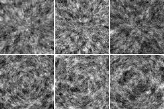
Fig. 1

Random draws from anisotropic Markov models. In the top row, the Markov model assumes stronger dependency between neighboring pixels in the radial than in angular direction, while in the bottom row, the roles of the directions are reversed. See text for a more detailed discussion

The just described construction of the smoothness prior is a particular instance of priors based on the assumption that the image is a Markov random field, (MRF). Similarly to the four-point average example, Markov random fields assume that the conditional probability distribution of a single pixel value X _jconditioned on the remaining image depends only on the neighbors of X _j,

$\displaystyle{\pi \left (x_{j}\mid x_{k},\,k\neq j\right ) =\pi \left (x_{j}\mid x_{k} \in N_{j}\right ),}$

where N _jis the list of neighbor pixels of X _j, such as the four adjacent pixels in the model (5). In fact, the Hammersley–Clifford theorem (see [5]) states that prior distributions of MRF models are of the form

$\displaystyle{\pi _{{\mathrm{prior}}}(x) \propto \mathrm{ exp}\left (-\sum _{j=1}^{N}V _{ j}(x)\right ),}$

where the function V _j(x) depends only on x _jand its neighbors. The simplest model in this family is a Gaussian white noise prior, where N _j= ∅ and $V _{j}(x) = x_{j}^{2}/(2\sigma ^{2})$ , that is,

$\displaystyle{\pi _{{\mathrm{prior}}}(x) \propto \mathrm{ exp}\left (-\frac{1} {2\sigma ^{2}}\|x\|^{2}\right ).}$

Observe that this prior assumes mutual independency of the pixels, which has qualitative repercussions on the images based on it.

There is no theoretical reason to restrict the MRFs to Gaussian fields, and in fact, some of the non-Gaussian fields have had a remarkable popularity and success in the imaging context. Two non-Gaussian priors are particularly worth mentioning here, the ℓ ¹-prior, where N _j= ∅ and V _j(x) = α | x _j|, that is,

$\displaystyle{\pi _{{\mathrm{prior}}}(x) \propto \mathrm{ exp}\left (-\alpha \|x\|_{1}\right ),\quad \|x\|_{1} =\sum _{ j=1}^{N}\vert x_{ j}\vert,}$

and the closely related total variation (TV) prior,

$\displaystyle{\pi _{{\mathrm{prior}}}(x) \propto \mathrm{ exp}\left (-\alpha {\mathrm{TV}}(x)\right ),\quad {\mathrm{TV}}(x) =\sum _{ j=1}^{N}V _{ j}(x),}$

with

$\displaystyle{V _{j}(x) = \frac{1} {2}\sum _{k\in N_{j}}\vert x_{j} - x_{k}\vert.}$

The former is suitable for imaging sparse images, where all but few pixels are believed to coincide with the background level that is set to zero. The latter prior is particularly suitable for blocky images, that is, for images consisting of piecewise smooth simple shapes. There is a strong connection to the recently popular concept of compressed sensing, see, for example, [11].

MRF priors, or priors with only local interaction between pixels, are by far the most commonly used priors in imaging. It is widely accepted and to some extent demonstrated (see [6] and the discussion in it) that the posterior density is sensitive to local properties of the prior only, while the global properties are predominantly determined by the likelihood. Thus, as far as the role of priors is concerned, it is important to remember that until the likelihood is taken into account, there is no connection with the measured data, hence no reason to believe that the prior should generate images that in the large scale resemble what we are looking for. In general, priors are usually designed to carry very general often qualitative and local information, which will be put into proper context with the guidance of the data through the integration with the likelihood. To demonstrate the local structure implied by different priors, in Fig. 2, we show some random draws from the priors discussed above.

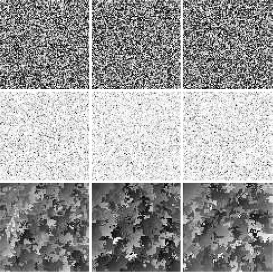
Fig. 2

Random draws from various MRF priors. Top row: white noise prior. Middle row: sparsity prior or ℓ ¹-prior with positivity constraint. Bottom row: total variation prior

Likelihood: Forward Model and Statistical Properties of Noise

If an image is worth a thousand words, a proper model of the noise corrupting it is worth at least a thousand more, in particular when the processing is based on the statistical methods. So far, the notion of noise has remained vague, and its role unclear. It is the noise, and in fact its statistical properties, that determines the likelihood density. We start by considering two very popular noise models.

Additive, nondiscrete noise: An additive noise model assumes that the data and the unknown are in a functional relation of the form

$\displaystyle{ y = F(x) + e, }$

(6)

where e is the noise vector. If the function F is linear, or it has been linearized, the problem simplifies to

$\displaystyle{ y = {\mathsf{A}}x + e. }$

(7)

The stochastic extension of (6) is

$\displaystyle{Y = F(X) + E,}$

where Y, X, and E are multivariate random vectors.

The form of the likelihood is determined not only by the assumed probability distributions of Y, X, and E but also by the dependency between pairs of these variables. In the simplest case, X and E are assumed to be mutually independent and the probability density of the noise vector known,

$\displaystyle{E \sim \pi _{{\mathrm{noise}}}(e),}$

resulting in a likelihood function of the form

$\displaystyle{\pi (y\mid x) \propto \pi _{{\mathrm{noise}}}\left (y - F(x)\right ),}$

which is one of the most commonly used in applications. A particularly popular model for additive noise is a Gaussian noise,

$\displaystyle{E \sim \mathcal{N}(0,\Sigma ),}$

where the covariance matrix $\Sigma$ is positive definite. Therefore, if we write $\Sigma ^{-1} = {\mathsf{D}}^{{\mathsf{T}}}{\mathsf{D}}$ , where D can be the Cholesky factor of $\Sigma ^{-1}$ or ${\mathsf{D}} = \Sigma ^{-1/2}$ , the likelihood can be written as

$\displaystyle\begin{array}{rcl} \pi (y\mid x)& \propto & \exp \left (-\frac{1} {2}(y - F(x))^{{\mathsf{T}}}\Sigma ^{-1}(y - F(x))\right ) \\ & =& \exp \left (-\frac{1} {2}\|{\mathsf{D}}(y - F(x))\|^{2}\right ). {}\end{array}$

(8)

In the general case where $$X$$

and E are not independent, we need to specify the joint density

$\displaystyle{(X,E) \sim \pi (x,e)}$

and the corresponding conditional density

$\displaystyle{\pi _{{\mathrm{noise}}}(e\mid x) = \frac{\pi (x,e)} {\pi _{{\mathrm{prior}}}(x)}.}$

In this case, the likelihood becomes

$\displaystyle{\pi (y\mid x) \propto \pi _{{\mathrm{noise}}}(y - F(x)\mid x).}$

This clearly demonstrates the problems which may arise if we want to adhere to the claim that “likelihood should be independent of the prior.” Because the interdependency of the image x and the noise is much more common than we might be inclined to believe, the independency of noise and signal is often in conflict with reality. An instance of such situation occurs in electromagnetic brain imaging using magnetoencephalography (MEG) or electroencephalography (EEG), when the eye muscle during a visual task acts as noise source but can hardly be considered as independent from the brain activation due to a visual stimulus. Another example related to boundary conditions will be discussed later on. Also, since the noise term should account not only for the exogenous measurement noise but also for the shortcomings of the model, including discretization errors, the interdependency is in fact a ubiquitous phenomenon too often neglected.

Most additive noise models assume that the noise follows a Gaussian distribution, with zero mean and given covariance. The computational advantages of a Gaussian likelihood are rather formidable and have been a great incentive to use Gaussian approximations of non-Gaussian densities. While it is commonplace and somewhat justified, for example, to approximate Poisson densities with Gaussian densities when the mean is sufficiently large [14], there are some important imaging applications where the statistical distribution of the noise must be faithfully represented in the likelihood.

Counting noise: The weakness of a signal can complicate the deblurring and denoising problem, as is the case in some image processing applications in astronomy [49, 57, 63], microscopy [45, 68], and medical imaging [29, 60]. In fact, in the case of weak signals, a charge-coupled device (CCD), instead of recording an integrated signal over a time window, counts individual photons or electrons. This leads to a situation where the noise corrupting the recorded signal is no longer exogenous but rather an intrinsic property of the signal itself, that is, the input signal itself is a random process with an unpredictable behavior. Under rather mild assumptions – stationarity, independency of increments, and zero probability of coincidence – it can be shown (see, e.g., [62]) that the counting signal follows a Poisson distribution. Consider, for example, the astronomical image of a very distant object, collected with an optical measurement device whose blurring is described by a matrix A. The classical description of such data would follow (7), with the error term collecting the background noise and the thermal noise of the device. The corresponding counting model is

$\displaystyle{y_{j} \sim \mathrm{ Poisson}\left (({\mathsf{A}}x)_{j} + b\right ),\mbox{ $y_{j}$, $y_{k}$ independent if $j\neq k$},}$

or, explicitly,

$\displaystyle{\pi (y\mid x) =\prod _{ j=1}^{m}\frac{(({\mathsf{A}}x)_{j} + b)^{y_{j}}} {(y_{j})!} {\mathrm{exp}}\left (-({\mathsf{A}}x)_{j} + b\right ),}$

where b ≥ 0 is a background radiation level, assumed known. Observe that while the data are counts, therefore integer numbers, the expectation need not to be.

Similar or slightly modified likelihoods can be used to model the positron emission tomography (PET) and single-photon emission computed tomography (SPECT) signals; see [29, 54].

The latter example above demonstrates clearly that the description of imaging problems as linear or nonlinear, without a specification of the noise model, in the context of statistical methods, does not play a significant role: Even if the expectation is linear, traditional algorithms for solving linear inverse problems are useless, although they may turn out to be useful within iterative solvers for solving locally linearized steps.

Maximum Likelihood and Fisher Information

When switching to a parametric non-Bayesian framework, the statistical inference problem amounts to estimating a deterministic parameter that identifies the probability distribution from which the observations are drawn. To apply this framework in imaging problems, the underlying image x, which in the Bayesian context was itself a random variable, can be thought of as a parameter vector that specifies the likelihood function,

$\displaystyle{f(y;x) =\pi (y\mid x),}$

as implied by the notation f(y; x) also.

In the non-Bayesian interpretation, a measure of how much information about the parameter x is contained in the observation is given in terms of the Fisher information matrix J,

$\displaystyle{ {\mathsf{J}}_{j,k} = {\mathsf{E}}\left \{ \frac{\partial \log f} {\partial x_{j}} \frac{\partial \log f} {\partial x_{k}}\right \} =\int \frac{\partial \log f(y;x)} {\partial x_{j}} \frac{\partial \log f(y;x)} {\partial x_{k}} f(y;x)dy. }$

(9)

In this context, the observation y only is a realization of a random variable Y, whose probability distribution is entirely determined by the distribution of the noise. The gradient of the logarithm of the likelihood function is referred to as the score, and the Fisher information matrix is therefore the covariance of the score.

Assuming that the likelihood is twice continuously differentiable and regular enough to allow the exchange of integration and differentiation, it is possible to derive another useful expression for the information matrix. It follows from the identity

$\displaystyle{ \frac{\partial \log f} {\partial x_{k}} = \frac{1} {f} \frac{\partial f} {\partial x_{k}}, }$

(10)

that we may write the Fisher information matrix as

$\displaystyle{{\mathsf{J}}_{j,k} =\int \frac{\partial \log f} {\partial x_{j}} \frac{\partial f} {\partial x_{k}}dy = \frac{\partial } {\partial x_{k}}\int \frac{\partial \log f} {\partial x_{j}}fdy -\int \frac{\partial ^{2}\log f} {\partial x_{j}\partial x_{k}}fdy.}$

Using the identity (10) with k replaced by j, we observe that

$\displaystyle{\int \frac{\partial \log f} {\partial x_{j}}fdy =\int \frac{\partial f} {\partial x_{j}}dy = \frac{\partial } {\partial x_{j}}\int fdy = 0,}$

since the integral of f is one, which leads us to the alternative formula

$\displaystyle{ {\mathsf{J}}_{j,k} = -\int \frac{\partial ^{2}\log f} {\partial x_{j}\partial x_{k}}fdy = -{\mathsf{E}}\left \{ \frac{\partial ^{2}\log f} {\partial x_{j}\partial x_{k}}\right \}. }$

(11)

The Fisher information matrix is closely related to non-Bayesian estimation theory. This will be discussed later in connection with maximum likelihood estimation.

Informative or Noninformative Priors?

Not seldom the use of priors in imaging applications is blamed for biasing the solution in a direction not supported by the data. The concern of the use of committal priors has led to the search of “noninformative priors” [39] or weak priors that would “let the data speak.”

The strength or weakness of a prior is a rather elusive concept, as the importance of the prior in Bayesian imaging is in fact determined by the likelihood: the more information we have about the image in data, the less has to be supplied by the prior. On the other hand, in imaging applications where the likelihood is built on very few data points, the prior needs to supply the missing information, hence has a much more important role. As pointed out before, it is a common understanding that in imaging applications, prior should carry small-scale information about the image that is missing from the likelihood that in turn carries information about the large-scale features and in that sense complements the data.

Adding Layers: Hierarchical Models

Consider the following simple denoising problem with additive Gaussian noise,

$\displaystyle{Y = X + N,\quad N \sim \mathcal{N}(0,\Sigma ),}$

with noise covariance matrix $\Sigma$ presumed known, whose likelihood model is tantamount to saying that

$\displaystyle{Y \mid X = x \sim \mathcal{N}(x,\Sigma ).}$

From this perspective, the denoising problem is reduced to estimating the mean of a Gaussian density in the non-Bayesian spirit, and the prior distribution is a hierarchical model, expressing the degree of uncertainty of the mean x.

Parametric models are common when defining the prior densities, but similarly to the above interpretation of the likelihood, the parameters are often poorly known. For example, when introducing a prior

$\displaystyle{X \sim \mathcal{N}(\theta,\Gamma )}$

with unknown θ, we are expressing a qualitative prior belief that “X differs from an unknown value by an error with a given Gaussian statistics,” which says very little about the values of X itself unless information about θ is provided. Similarly as in the denoising problem, it is natural to augment the prior with another layer of information concerning the parameter θ. This layering of the inherent uncertainty is at the core of hypermodels, or Bayesian hierarchical models. Hierarchical models are not restricted to uncertainties in the prior, but can be applied to lack of information of the likelihood model as well.

In hierarchical models, both the likelihood and the prior may depend on additional parameters,

$\displaystyle{\pi (y\mid x) \rightarrow \pi (y\mid x,\gamma ),\quad \pi _{{\mathrm{prior}}}(x) \rightarrow \pi _{{\mathrm{prior}}}(x\mid \theta ),}$

with both parameters γ and θ poorly known. In this case, it is natural to augment the model with hyperpriors. Assuming for simplicity that the parameters γ and θ are mutually independent so that we can define the hyperprior distributions π ₁(γ) and π ₂(θ), the joint probability distribution of all the unknowns is

$\displaystyle{\pi (x,y,\theta,\gamma ) =\pi (y\mid x,\gamma )\pi _{{\mathrm{prior}}}(x\mid \theta )\pi _{1}(\gamma )\pi _{2}(\theta ).}$

From this point on, the Bayesian inference can proceed along different paths. It is possible to treat the hyperparameters as nuisance parameters and marginalize them out by computing

$\displaystyle{\pi (x,y) =\int \int \pi (x,y,\theta,\gamma )d\theta d\gamma }$

and then proceed as in a standard Bayesian inference problem. Alternatively, the hyperparameters can be included in the list of unknowns of the problem and their posterior density

$\displaystyle{\pi (\xi \mid y) = \frac{\pi (x,y,\theta,\gamma )} {\pi (y)},\quad \xi = \left [\begin{array}{@{}c@{}} x\\ \theta \\ \gamma \end{array} \right ]}$

needs to be explored. The estimation of the hyperparameters can be based on the optimization or on the evidence, as will be illustrated below with a specific example.

To clarify the concept of a hierarchical model itself, we consider some examples where hierarchical models arise naturally.

Blind deconvolution: Consider the standard deblurring problem defined in section “Imaging Problems.” Usually, it is assumed that the blurring kernel A is known, and the likelihood, with additive Gaussian noise with covariance $\Sigma$ , becomes

$\displaystyle{ \pi (y\mid x) \propto \mathrm{ exp}\left (-\frac{1} {2}(y -{\mathsf{A}}x)^{{\mathsf{T}}}\Sigma ^{-1}(y -{\mathsf{A}}x)\right ). }$

(12)

In some cases, although A is poorly known, its parametric expression is known and the uncertainty only affects the values of some parameters, as is the case when the shape of the continuous convolution kernel a(r − s) is known but the actual width is not. If we express the kernel a as a function of a width parameter,

$$$\displaystyle{a(r - s) = a_{\gamma }(r - s) = \frac{1} {\gamma } a_{1}(\gamma (r - s)),\quad \gamma > 0,}$$” src=”/wp-content/uploads/2016/04/A183156_2_En_53_Chapter_Equaq.gif”></DIV></DIV></DIV>and denote by <SPAN class=EmphasisFontCategorySansSerif>A</SPAN> <SUB><SPAN class=EmphasisTypeItalic>γ</SPAN> </SUB>the corresponding discretized convolution matrix, the likelihood becomes<br /> <DIV id=Equar class=Equation><br /> <DIV class=EquationContent><br /> <DIV class=MediaObject><IMG alt=$

and additional information concerning γ, for example, bound constraints, can be included via a hyperprior density.

The procedure just outlined can be applied to many problems arising from adaptive optics imaging in astronomy [52]; while the uncertainty in the model is more complex than in the explanatory example above, the approach remains the same.

Conditionally Gaussian hypermodels: Gaussian prior models are often criticized for being a too restricted class, not being able to adequately represent prior beliefs concerning, for example, the sparsity or piecewise smoothness of the solution. The range of qualitative features that can be expressed with normal densities can be considerably expanded by considering conditionally Gaussian families instead. As an example, consider the problem of finding a sparse image from linearly blurred noisy copy of it. The likelihood model in this case may be written as in (12). To set up an appropriate prior, consider a conditionally Gaussian prior

$\displaystyle\begin{array}{rcl} \pi _{{\mathrm{prior}}}(x\mid \theta )& \propto & \left ( \frac{1} {\theta _{1}\ldots \theta _{N}}\right )^{1/2}{\mathrm{exp}}\left (-\frac{1} {2}\sum _{j=1}^{N}\frac{x_{j}^{2}} {\theta _{j}} \right ) \\ & =& {\mathrm{exp}}\left (-\frac{1} {2}\sum _{j=1}^{N}\left [\frac{x_{j}^{2}} {\theta _{j}} +\log \theta _{j}\right ]\right ).{}\end{array}$

(13)

If $\theta _{j} =\theta _{0} = \text{constant}$ , we obtain the standard white noise prior which cannot be expected to favor sparse solutions. On the other hand, since θ _jis the variance of the pixel X _j, sparse images correspond to vectors θ with most of the components close to zero. Since we do not know a priori which of the variances should significantly differ from zero, when choosing a stochastic model for θ, it is reasonable to select a hyperprior that favors sparsity without actually specifying the location of the outliers. Two distributions that are particularly well suited for this are the gamma distribution,

$$$\displaystyle{\theta _{j} \sim \text{Gamma}(k,\theta _{0}),\quad k,\theta _{0} > 0,\quad \pi (\theta _{j}) =\theta _{ j}^{k-1}{\mathrm{exp}}\left (-\frac{\theta _{j}} {\theta _{0}}\right ),}$$” src=”/wp-content/uploads/2016/04/A183156_2_En_53_Chapter_Equas.gif”></DIV></DIV></DIV>and the <SPAN class=EmphasisTypeItalic>inverse gamma distribution</SPAN>,<br /> <DIV id=Equat class=Equation><br /> <DIV class=EquationContent><br /> <DIV class=MediaObject><IMG alt=$ 0,\quad \pi (\theta _{j}) =\theta _{ j}^{-k-1}{\mathrm{exp}}\left (-\frac{\theta _{0}} {\theta _{j}}\right ).}$$” src=”/wp-content/uploads/2016/04/A183156_2_En_53_Chapter_Equat.gif”>

The parameters k and θ ₀ are referred to as the shape and the scaling, respectively. The inverse gamma distribution corresponds to assuming that the precision , defined as 1∕θ _j, is distributed according to the gamma distribution Gamma(k, 1∕θ ₀). The computational price of introducing hyperparameters is that instead of one image x, we need to estimate the image x and its variance image θ. Fortunately, for conditionally Gaussian families, there are efficient algorithms for computing these estimates, which will be discussed in the section concerning algorithms.

The hyperprior based on the gamma distribution, in turn, contains parameters (k and θ ₀) to be determined. Nothing prevents us from defining another layer of hyperpriors concerning these values. It should be noted that in hierarchical models, the selection of the parameters higher up in the hierarchy tends to have less direct effect on the parameters of primary interest. Since this last statement has not been formally proved to be true, it should be considered as a piece of computational folklore.

Conditionally Gaussian hypermodels have been successfully applied in machine learning [66], in electromagnetic brain activity mapping [16], and in imaging applications for restoring blocky images [15]. Recently, their use in compressed sensing has been proposed [40].

4 Numerical Methods and Case Examples

The solution of an imaging inverse problem in the statistical framework is the posterior probability density. Because this format of the solution is not practical for most applications, it is common to summarize the distribution in one or a few images. This leads to the challenging problem of exploring the posterior distributions and finding single estimators supported by the distribution.

Estimators

In this section, we review some of the commonly used estimators and subsequently discuss some of the popular algorithms suggested in the literature to compute the corresponding estimates.

Prelude: Least Squares and Tikhonov Regularization

In the case where the forward model is linear, the problem of estimating an image from a degraded, noisy recording is equivalent in a determinist setting to looking for a solution of a linear system of equations of the form

$\displaystyle{ {\mathsf{A}}x = y, }$

(14)

where the right-hand side is corrupt by noise. When A is not a square matrix and/or it is ill conditioned, one needs to specify what a “solution” means. The most straightforward way is to specify it as a least squares solution.

There is a large body of literature, and a wealth of numerical algorithms, for the solution of large-scale least squares problems arising from problems similar to imaging applications (see, e.g., [9]). Since dimensionality alone makes these problems computationally very demanding, they may require an unreasonable amount of computer memory and operations unless a compact representation of the matrix A can be exploited. Many of the available algorithms make additional assumptions about either the underlying image or the structure of the forward model regardless of whether there is a good justification.

In a determinist setting, the entries of the least squares solution of (14) with a right-hand side corrupted by noise are not necessarily in the gray-scale range of the image pixels. Moreover, the inherent ill conditioning of the problem, which varies with the imaging modality and the conditions under which the observations were collected, usually requires reqularization, see, for example, [4, 33, 34, 41]. A standard regularization method is to replace the original ill-posed least squares problem by a nearby well-posed problem by introducing a penalty term to avoid that the computed solution is dominated by amplified noise components, reducing the problem to minimizing a functional of the form

$\displaystyle{ T(x) =\| {\mathsf{A}}x - y\|^{2} +\alpha J(x), }$

(15)

where J(x) is the penalty functional and α > 0 is the regularization parameter. The minimizer of the functional (15) is the Tikhonov regularized solution . The type of additional information used in the design of the penalty term may include upper bounds on the norm of the solution or of its derivatives, nonnegative constraints for its entries, or bounds on some of the components. Often, expressing characteristics that are expected of the sought image in qualitative terms is neither new nor difficult: the translation of these beliefs into mathematical terms and their implementation is a more challenging step.

Maximum Likelihood and Maximum A Posteriori

We begin with the discussion of the maximum likelihood estimator in the framework of non-Bayesian statistics and denote by x a deterministic parameter determining the likelihood distribution of the data, modeled as a random variable. Let $\hat{x} =\hat{ x}(y)$ denote an estimator of x, based on the observations y. Obviously, $\hat{x}$ is also a random variable, because of its dependency on the stochastic observations y; moreover, it is an unbiased estimator if

$\displaystyle{{\mathsf{E}}\left \{\hat{x}(y)\right \} = x,}$

that is, if, in the average, it returns the exact value. The covariance matrix C of an unbiased estimator therefore measures the statistical variation around the true value,

$\displaystyle{{\mathsf{C}}_{j,k} = {\mathsf{E}}\left \{(\hat{x}_{j} - x_{j})(\hat{x}_{k} - x_{k})\right \},}$

thus the name mean square error. Evidently, the smaller the mean square error, for example, in the sense of quadratic forms, the higher the expected fidelity of the estimator. The Fisher information matrix (9) gives a lower bound for the covariance matrix of all unbiased estimators. Assuming that J is invertible, the Cramér–Rao lower bound states that for an unbiased estimator,

$\displaystyle{{\mathsf{J}}^{-1} \leq {\mathsf{C}}}$

in the sense of quadratic forms, that is, for any vector

$\displaystyle{u^{{\mathsf{T}}}{\mathsf{J}}^{-1}u \leq u^{{\mathsf{T}}}{\mathsf{C}}u.}$

An estimator is called efficient if the error covariance reaches the Cramér–Rao bound.

The maximum likelihood estimator $\hat{x}_{{\mathrm{ML}}}(y)$ is the maximizer of the function x ↦ f(x; y), and in practice, it is found by locating the zero(s) of the score,

$\displaystyle{\nabla _{x}\log f(x;y) = 0 \Rightarrow x =\hat{ x}_{{\mathrm{ML}}}(y).}$