(1)
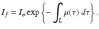
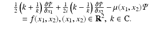
We denote by I o the initial intensity of a gamma ray and by I f the measured intensity after undergoing attenuation through tissue of length L; the above equation can be written in the form
(2)
Let f(x 1, x 2) denote the distribution in the tissue of the radioactive material under consideration, and let L(x) denote the part of the ray from the tissue to the detector. Then, in SPECT, it is assumed that the following integral, I SPECT, is known from the measurements:
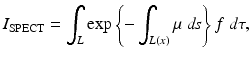
where the integral is measured over a finite number of lines L. Equation (3) is valid under the following assumptions:
(3)
(a)
The lines L are lying within a specified imaging plane,
(b)
The imaging system has perfect imaging characteristics,
(c)
The detector is collimated and can pick up radiation only along the straight lines L,
(d)
The collimator has an infinitely high spatial resolution,
(f)
There is no scatter radiation in the object.
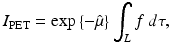


In order to derive Eq. (4) from Eq. (3), we recall that positrons eject particles pairwise in opposite directions, and in PET the radiation in opposite directions is measured simultaneously. Thus,
and Eq. (3) becomes Eq. (4).
(6)
In both PET and SPECT, a projection is formed by combining a set of line integrals along a line L. Here, we will consider parallel-ray integrals at a specific angle θ, i.e., we will assume a parallel-beam geometry.
We recall that the Radon transform of the X-ray attenuation coefficient denoted by μ CT is measured via computed tomography (CT). Using the values of μ CT, it is possible to estimate μ(x 1, x 2) by appropriate scaling (this is necessary due to the energy difference between X-rays and gamma rays).
Equation (4) implies that in PET one needs to reconstruct a function f from the knowledge of its Radon transform denoted by  ,
,

where  can be computed via
Hence, both CT and PET involve the computation of a function from the knowledge of its Radon transform. More specifically, in CT one needs to compute μ CT from the knowledge of  , whereas in PET one needs to compute f from the knowledge of
  . The relevant formula, known as the inverse Radon transform, is given by
where J is defined in terms of  by
by
and throughout this chapter, ∮ denotes the principal value integral.
,(7)
can be computed via(8)
, whereas in PET one needs to compute f from the knowledge of . The relevant formula, known as the inverse Radon transform, is given by(9)
by(10)
Let  denote the right-hand side (RHS) of Eq. (3). We call
  the attenuated Radon transform of f (with attenuation specified by the given function μ). Hence, SPECT involves the computation of a function f from the knowledge of its attenuated Radon transform
  and of the function μ. The relevant formula is known as the inverse attenuated Radon transform (IART).
denote the right-hand side (RHS) of Eq. (3). We call the attenuated Radon transform of f (with attenuation specified by the given function μ). Hence, SPECT involves the computation of a function f from the knowledge of its attenuated Radon transform and of the function μ. The relevant formula is known as the inverse attenuated Radon transform (IART). According to Eq. (9), the numerical implementation of the inverse Radon transform involves the computation of the Hilbert transform (Hf)(ρ) of a given function f(ρ), where
The most well-known method for this computation uses the fast Fourier transform technique, exploiting the fact that the Hilbert transform is a convolution. The application of this method to the computation of the inverse Radon transform is called filtered backprojection (FBP).
(11)
Most PET systems have options for both FBP and Ordered Subset Expectation Maximization (OSEM), which is the predominant iterative technique.
The analytical approach to SPECT requires the numerical implementation of the IART. However, since no analytical formula was available until recently for the IART, currently the FBP implementation to SPECT generally makes the crude approximation of μ = 0 or incorporates a uniform attenuation map [6]. On the other hand, since OSEM is based on an iterative statistical approach, it does not require the analytical inversion formula, and hence OSEM considers the actual values of μ. Hence, in SPECT, OSEM produces more accurate images than FBP. However, for several reasons including speed (1 s vs. 2.5 min for a typical study), FBP is still used extensively. Indeed, most SPECT systems have options for both FBP and OSEM, and both are used clinically. Actually, some clinicians prefer FBP for quantification.
In this review, we will discuss an alternative approach for computing the Hilbert transform. This approach, in contrast to FBP which is formulated in the Fourier space, is formulated in the physical space, and it is based on “custom-made” cubic splines. We will refer to the application of this approach to the computation of the inverse Radon transform and to the IART as spline reconstruction technique (SRT) for PET and SRT for SPECT, respectively.
The results of rigorous studies comparing FBP with SRT for PET are published in [7]. In these studies, which use both simulated and real data, by employing a variety of image quality measures, including contrast and bias, it is established that SRT has certain advantages in comparison with FBP. As a result of these studies, SRT is now included in STIR (Software for Tomographic Image Reconstruction) [8], which is a widely used open-source software library in tomographic imaging (FBP and SRT are the only algorithms based on analytical formulae which are incorporated in STIR).
Rigorous studies comparing SRT for SPECT with FBP and OSEM are work in progress. Preliminary results suggest that SRT is preferable to FBP and also that SRT is comparable with OSEM; see Fig. 1 [9].
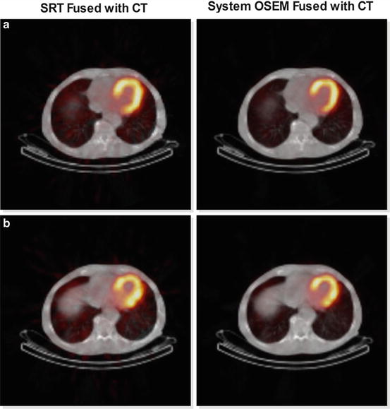
Fig. 1
Reconstructions of two consecutive slices (a and b) of the myocardium acquired with SPECT fused with CT scan. The images on the right are obtained by the currently used commercial software and on the left with SRT
The clinical importance of PET and SPECT, as well as the mathematical formulation of the inverse Radon transform and of the IART, is further discussed in the following section. A new method for deriving transforms in one and two dimensions was introduced in [10]. Using this method, both the inverse Radon transform and the IART are derived in Sect. 3. The SRT for PET is presented in Sect. 4, and the studies of Kastis et al. [7] comparing SRT with FBP for PET are reviewed in Sect. 5. SRT for SPECT is briefly discussed in Sect. 6.
2 Background
The Importance of PET and SPECT
In 1964, the research group of Dr. David E. Kuhl, known as the “Father of Emission Tomography,” developed the Mark II SPECT series, which is a single-emission computed tomography camera. Using this unit, this group succeeded in producing the world’s first tomographic images of the human body. This achievement was considerably earlier than Godfrey Hounsfield’s development of the X-ray CT device in 1972. A crucial element in the evolution of emission tomography was the choice of the radioisotope injected in the patient. An important such class is those radioisotopes that emit positrons. An emitted positron almost immediately combines with a nearby electron; they annihilate each other, emitting in the process two gamma rays traveling in nearly opposite directions. PET cameras detect these gamma rays.
FDG (18F-2-deoxy-2-fluoro-D-glucose) is the most suitable positron emitter that can be used with humans. It is a deoxyglucose analog with the normal hydroxyl group in the glucose molecule substituted with the radioactive isotope18F. FDG is taken up by high-glucose-using cells, and it is metabolically trapped following phosphorylation by the hexokinase enzyme [11]. Thus, the measurement of the positron-emitting18F provides a quantitative measure of the glucose consumed in the corresponding tissue. Glucose metabolism in cancerous tissue is higher than in normal tissue. Thus, PET-CT devices are proving to be highly effective in the early detection of cancer. For example, among 91 patients with non-small-cell lung cancer, 38 pathologically confirmed mediastinal lymph node metastases were missed by CT, whereas among 98 similar patients, only 21 metastases were missed by PET-CT [12] (this means that in the former case, there were 38 futile thoracotomies, whereas in the latter case, there were only 21). Furthermore, using more specific positron emitters, it is possible to obtain additional useful information. For example, using F-fluoro-17-β-estradiol, it is possible to access in vivo the density of estrogen receptors as well as to monitor the response of the treatment for estrogen receptor-positive breast cancer. Similarly, using18F-annexin V, it is possible to follow tumor cell apoptosis (death) in vivo, as well as to monitor treatment response to various cancer types. It should also be noted that PET-CT is useful for prognosis. For example, the 2-year failure-free survival rate of patients with positive scans after chemotherapy treatment for early-stage Hodgkin’s lymphoma was 69 %, as compared with 95 % of patients with negative scans [13].
In addition to oncology, PET is now used in several other areas of medicine, including cardiology and neurology. As an example of the usefulness of PET in neurology, we note that PET with the use of the Pittsburgh compound B(PIB) can be used to quantify the concentration of amyloid-beta (Aβ) deposition in the brain, a precursor of Alzheimer’s disease [14].
SPECT is used extensively in cardiology, oncology, and neurology. In cardiology, SPECT is part of the common stress-testing procedures for the evaluation of chest pain [15]. As an example of the use of SPECT in oncology, we mention the study in [16], where lymphoscintigraphy was performed using SPECT-CT to establish a preoperative road map of lymph nodes that are at risk for metastatic melanoma and to facilitate intraoperative identification of the “sentinel” nodes (the rationale for sentinel-node biopsy relies on the concept that different regions of the skin have specific patterns of lymphatic drainage to the regional nodes, and for a given region of the skin, there exists at least a specific node, the sentinel node, in which lymphatic vessels drain first, and it is this node the most likely first site of metastasis).
In neurology, SPECT can be used to image the distribution of the blood flow in the brain, and this has been used in a plethora of pathological situations. Furthermore, by employing specific radioisotopes, it is possible to obtain useful information about several diseases. For example, using SPECT with123I-labeled CIT, it is shown in [17] that although levodopa treatment is highly effective as dopamine replacement in Parkinson’s disease, this treatment apparently downregulates the endogenous dopamine transporters.
The Mathematical Foundation of the IART
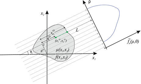
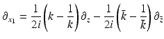
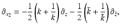
Consider a line L specified by two real numbers ρ and θ, where −∞ < ρ < ∞ and 0 ≤ θ < 2π (Fig. 2). A unit vector along this line is given by
A unit vector perpendicular to L is given by
A point x on this line can be expressed in the form
Hence,
Solving these equations for (τ, ρ) in terms of (x 1, x 2, θ), we find
Writing (x 1, x 2) in terms of the local coordinates (ρ, θ), it follows that the equation defining the Radon transform,  , of a function f takes the form
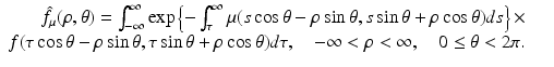
Similarly, the following equation provides the definition of the attenuated Radon transform,  (with attenuation specified by μ), of a function f:
(12)
(13)
(14)
(15)
(16)
(17)
(18)
, of a function f takes the form(19)
(with attenuation specified by μ), of a function f:(20)
Fig. 2
Parallel-beam projections through an object with attenuation coefficient μ(x 1, x 2). The local and Cartesian coordinates of the mathematical formulation are indicated
The inverse Radon transform, expressing f in terms of  , is given by Eqs. (9) and (10). Similarly, the IART, expressing f in terms of
  and μ, is given by
where the function J is defined by
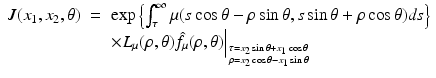
and the operator L μ (ρ, θ) is defined by
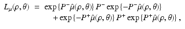
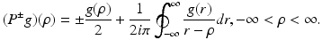
with  denoting the Radon transform of μ(x 1, x 2) and the operators P ± denoting the usual projection operators in the variable ρ, i.e.,
, is given by Eqs. (9) and (10). Similarly, the IART, expressing f in terms of and μ, is given by(21)
(22)
(23)
denoting the Radon transform of μ(x 1, x 2) and the operators P ± denoting the usual projection operators in the variable ρ, i.e.,(24)
A General Methodology for Constructing Transform Pairs
The study of nonlinear integrable equations led to the emergence of a general method for deriving transform pair in one and two dimensions [10]. In particular, using this method, it was shown in [10] that the two-dimensional Fourier transform of a function u(x 1, x 2) can be constructed via the spectral analysis of the equation
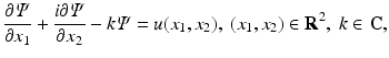
where  is a scalar function and bar denotes complex conjugate.
(25)
is a scalar function and bar denotes complex conjugate.R. Novikov and one of the authors re-derived in [18] the Radon transform by performing the spectral analysis of the equation
Although the Radon transform can be derived in a much simpler way by using the two-dimensional Fourier transform, the advantage of the derivation of [18] was demonstrated later by Novikov [19] who showed that the inverse attenuated Radon transform can be derived by applying a similar analysis to the following slight generalization of Eq. (26):
(26)
(27)
3 The Inverse Radon Transform and the Inverse Attenuated Radon Transform
In what follows, we discuss an algorithmic approach for the construction of a transform pair  . The relevant analysis, which is usually referred to as spectral analysis, involves two main steps: (i) solve a given eigenvalue equation in terms of f. If k denotes the eigenvalue parameter, this involves constructing a solution Ψ of the given eigenvalue equation which is bounded for all complex values of k. This problem will be referred to as the direct problem. (ii) Using the fact that Ψ is bounded for all complex k, construct an alternative representation of Ψ which (instead of depending on f) depends on some “spectral function” of f denoted by
  . This problem will be referred to as the inverse problem.
. The relevant analysis, which is usually referred to as spectral analysis, involves two main steps: (i) solve a given eigenvalue equation in terms of f. If k denotes the eigenvalue parameter, this involves constructing a solution Ψ of the given eigenvalue equation which is bounded for all complex values of k. This problem will be referred to as the direct problem. (ii) Using the fact that Ψ is bounded for all complex k, construct an alternative representation of Ψ which (instead of depending on f) depends on some “spectral function” of f denoted by . This problem will be referred to as the inverse problem.It turns out that the inverse problem gives rise to certain problems in complex analysis known as the Riemann-Hilbert and the d-bar problems. Indeed, for certain eigenvalue problems, the function Ψ is sectionally analytic in k, i.e., it has different representations in different domains of the complex k-plane, and each of these representations is analytic. In this case, if the “jumps” of these representations across the different domains can be expressed in terms of  , then it is possible to reconstruct Ψ as the solution of a Riemann-Hilbert problem which is uniquely defined in terms of
  . However, for a large class of eigenvalue problems, there exists a domain in the complex k-plane where Ψ is not analytic. In this case, if
  can be expressed in terms of
  , then Ψ can be reconstructed through the solution of a d-bar problem which is uniquely defined in terms of
  .
.
, then it is possible to reconstruct Ψ as the solution of a Riemann-Hilbert problem which is uniquely defined in terms of . However, for a large class of eigenvalue problems, there exists a domain in the complex k-plane where Ψ is not analytic. In this case, if can be expressed in terms of , then Ψ can be reconstructed through the solution of a d-bar problem which is uniquely defined in terms of .We recall that the classical derivation of transform pairs involves the integration in the complex k-plane of an appropriate Green’s function. However, this derivation is based on the assumption that the Green’s function is an analytic function of k and it also assumes completeness. The assumption of analyticity corresponds to the case that Ψ is sectionally analytic. Therefore, the approach reviewed here has the advantage that not only it provides a simpler approach to deriving classical transforms avoiding the problem of completeness, but also it can be applied to problems that the associated Green’s function is not an analytic function of k.
In addition to the construction of the Inverse attenuated Radon transform, the approach reviewed here has led to the construction of the X-ray fluorescence computed tomography [20].
The Construction of the Inverse Radon Transform
Let S(R 2) denote the space of Schwartz functions. Define the Radon transform  of the function
 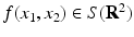 by Eq. (19). Then, for all (x 1, x 2) ∈ R 2, f(x 1, x 2) is given by Eq. (9).
of the function by Eq. (19). Then, for all (x 1, x 2) ∈ R 2, f(x 1, x 2) is given by Eq. (9).We will derive the Radon transform pair by performing the spectral analysis of the eigenvalue Eq. (26). In order to solve the direct problem, we first simplify Eq. (26) by introducing a change of variables from (x 1, x 2) to  , where z is defined by
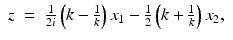
and  follows via complex conjugation, i.e.,
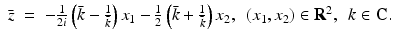 Using the identities
and
Eq. (26) becomes
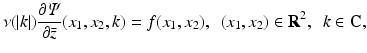
where the function ν( | k | ) is defined by
We supplement Eq. (31) with the boundary condition

In order to solve Eqs. (31) and (33), we will use the Pompeiu formula, namely,
where ∂ D denotes the boundary of the domain D. Using this formula, we find
Hence, using the identity
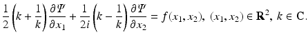
it follows that for all (x 1, x 2) ∈ R 2 and k ∈ C, | k | ≠ 1, Ψ satisfies
If k is either inside or outside the unit circle, the only dependence of Ψ on k is through z ′ and z; thus, Ψ is a sectionally analytic function with a “jump” across the unit circle of the complex k-plane. Equation (37) provides the solution of the direct problem.
, where z is defined by(28)
follows via complex conjugation, i.e.,(29)
(30)
(31)
(32)
(33)
(34)
(35)
(36)
(37)
In order to solve the inverse problem, we will formulate a Riemann-Hilbert problem in the complex k-plane. In this respect, we note that Eq. (37) implies
Furthermore, we will show that for all (x 1, x 2) ∈ R 2, Ψ satisfies the following “jump” condition:

where H denotes the Hilbert transform in the variance ρ defined in Eq. (11). This equation is a direct consequence of the following equations: let Ψ + and Ψ − denote the limits of Ψ as k approaches the unit circle from inside and outside, i.e.,
Then, for all (x 1, x 2) ∈ R 2,
where P ± denote the usual projectors in the variable ρ, i.e.,
and F denotes f in the coordinates (ρ, τ, θ), i.e.,

Indeed, in order to derive Eq. (41), we note that the definition of z implies
Let
and similarly for (k −∓ 1∕k −).
(38)
(39)
(40)
(41)
(42)
(43)
(44)
(46)
Hence, for computing Ψ ± via Eq. (37


Related posts:

Stay updated, free articles. Join our Telegram channel
Full access? Get Clinical Tree
