is represented by data  according to an observation model, called also forward model
(1)
 is a (linear or nonlinear) transform. When u is an m × n image, its pixels are arranged columnwise into a p-length real vector, where p = mn and the original u[i, j] is identified with
 ![$$u[(i - 1)m + j]$$](/wp-content/uploads/2016/04/A183156_2_En_5_Chapter_IEq4.gif) . Some typical applications are, for instance, denoising, deblurring, segmentation, zooming and super-resolution, reconstruction in inverse problems, coding and compression, feature selection, and compressive sensing. In all these cases, recovering a good estimate
. Some typical applications are, for instance, denoising, deblurring, segmentation, zooming and super-resolution, reconstruction in inverse problems, coding and compression, feature selection, and compressive sensing. In all these cases, recovering a good estimate  for u o needs to combine the observation along with a prior and desiderata on the unknown u o . A common way to define such an estimate is
(2)
(3)
 is called an energy (or an objective),
  is a set of constraints,
  is a data-fidelity term,
  brings prior information on u o , and β > 0 is a parameter which controls the trade-off between
  and
and  .
.The term  ensures that
  satisfies (1) quite faithfully according to an appropriate measure. The noise n is random and a natural way to derive
  from (1) is to use probabilities; see, e.g., [7, 32, 37, 56]. More precisely, if
  is the likelihood of data v, the usual choice is
For instance, if A is a linear operator and  where n is additive independent and identically distributed (i.i.d.) zero-mean Gaussian noise, one finds that
This remains quite a common choice partly because it simplifies calculations.
ensures that satisfies (1) quite faithfully according to an appropriate measure. The noise n is random and a natural way to derive from (1) is to use probabilities; see, e.g., [7, 32, 37, 56]. More precisely, if is the likelihood of data v, the usual choice is(4)
where n is additive independent and identically distributed (i.i.d.) zero-mean Gaussian noise, one finds that(5)
The role of  in (3) is to push the solution to exhibit some a priori known or desired features. It is called prior or regularization or penalty term. In many image processing applications,
  is of the form
where for any i ∈ { 1, …, r},  , for s an integer
  , are linear operators and
  is usually the ℓ 1 or the ℓ 2 norm. For instance, the family
  can represent the discrete approximation of the gradient or the Laplacian operator on u or the finite differences of various orders or the combination of any of these with the synthesis operator of a frame transform or the vectors of the canonical basis of
  . Note that s = 1 if {D i } are finite differences or a discrete Laplacian; then
 And if {D i } are the basis vectors of
  , one has ϕ( | D i u | ) = ϕ( | u[i] | ). In (6),
  is quite a “general” function, often called a potential function (PF). A very standard assumption is that
in (3) is to push the solution to exhibit some a priori known or desired features. It is called prior or regularization or penalty term. In many image processing applications, is of the form(6)
, for s an integer , are linear operators and is usually the ℓ 1 or the ℓ 2 norm. For instance, the family can represent the discrete approximation of the gradient or the Laplacian operator on u or the finite differences of various orders or the combination of any of these with the synthesis operator of a frame transform or the vectors of the canonical basis of . Note that s = 1 if {D i } are finite differences or a discrete Laplacian; then, one has ϕ( | D i u | ) = ϕ( | u[i] | ). In (6), is quite a “general” function, often called a potential function (PF). A very standard assumption is thatH1
 is proper, lower semicontinuous (l.s.c.) and increasing on
  , with ϕ(t) > ϕ(0) for any t > 0.
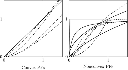
 Some typical examples for ϕ are given in Table 1 and their plots in Fig. 1.
Table 1
Commonly used PFs  where α > 0 is a parameter. Note that among the nonconvex PFs, (f8), (f10), and (f12) are coercive, while the remaining PFs, namely, (f6), (f7), (f9), (f11), and (f13), are bounded. And all nonconvex PFs with ϕ′(0+) > 0 are concave on
  . Recall that (f6) is the discrete equivalent of the Mumford-Shah (MS) prior [17, 72]
where α > 0 is a parameter. Note that among the nonconvex PFs, (f8), (f10), and (f12) are coercive, while the remaining PFs, namely, (f6), (f7), (f9), (f11), and (f13), are bounded. And all nonconvex PFs with ϕ′(0+) > 0 are concave on . Recall that (f6) is the discrete equivalent of the Mumford-Shah (MS) prior [17, 72]Convex PFs | |||
|---|---|---|---|
 | ϕ′(0+) > 0 | ||
(f1) | 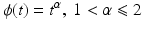 | (f5) | ϕ(t) = t |
(f2) | 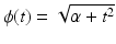 | ||
(f3) | 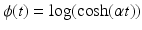 | ||
(f4) | 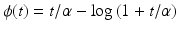 | ||
Nonconvex PFs | |||
 | ϕ′(0+) > 0 | ||
(f6) | ϕ(t) = min{α t 2, 1} | (f10) | ϕ(t) = t α , 0 < α < 1 |
(f7) |  | (f11) |  |
(f8) | 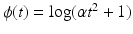 | (f12) |  |
(f9) |  | (f13) |  |

Remark 1.
If ϕ′(0+) > 0 the function t → ϕ( | t | ) is nonsmooth at zero in which case  is nonsmooth on
 ![$$\cup _{i=1}^{r}[w \in \mathbb{R}^{p}:\mathrm{ D}_{i}w = 0]$$](/wp-content/uploads/2016/04/A183156_2_En_5_Chapter_IEq43.gif) . Conversely,
. Conversely,  leads to a smooth at zero t → ϕ( | t | ). With the PF (f13),
  leads to the counting function, commonly called the ℓ 0-norm.
is nonsmooth on . Conversely, leads to a smooth at zero t → ϕ( | t | ). With the PF (f13), leads to the counting function, commonly called the ℓ 0-norm.For the human vision, an important requirement is that the prior  promotes smoothing inside homogeneous regions but preserves sharp edges. According to a fine analysis conducted in the 1990s and summarized in [7], ϕ preserves edges if H1 holds as if H2, stated below, holds true as well:
promotes smoothing inside homogeneous regions but preserves sharp edges. According to a fine analysis conducted in the 1990s and summarized in [7], ϕ preserves edges if H1 holds as if H2, stated below, holds true as well:H2

This assumption is satisfied by all PFs in Table 1 except for (f1) in case if α = 2. Note that there are numerous other heuristics for edge preservation.
Background
Energy minimization methods, as described here, are at the crossroad of several well-established methodologies that are briefly sketched below.
Bayesian maximum a posteriori (MAP) estimation using Markov random field (MRF) priors. Such an estimation is based on the maximization of the posterior distribution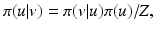 where π(u) is the prior model for u o and Z = π(v) can be seen as a constant. Equivalently,
  minimizes with respect to u the energy
Identifying these first term above with
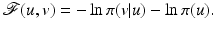
 and the second one with
  shows the basis of the equivalence. Classical papers on MAP energies using MRF priors are [14–16, 20, 51, 56]. Since the pioneering work of Geman and Geman [56], various nonconvex PFs ϕ were explored in order to produce images involving neat edges; see, e.g., [54, 55, 65]. MAP energies involving MRF priors are also considered in many books, such as [32, 53, 64]. For a pedagogical account, see [96].
Regularization for ill-posed inverse problems was initiated in the book of Tikhonov and Arsenin [93] in 1977. The main idea can be stated in terms of the stabilization of this kind of problems. Useful textbooks in this direction are, e.g., [61, 69, 94] and especially the recent [91]. This methodology and its most recent achievements are nicely discussed from quite a general point of view in Chapter Regularization Methods for Ill-Posed Problems in this handbook.
Variational methods are related to PDE restoration methods and are naturally developed for signals and images defined on a continuous subset , d = 1, 2, …; for images d = 2. Originally, the data-fidelity term is of the form (5) for A = Id and
  , where ϕ is a convex function as those given in Table 1 (top). Since the beginning of the 1990s, a remarkable effort was done to find heuristics on ϕ that enable to recover edges and breakpoints in restored images and signals while smoothing the regions between them; see, e.g., [7, 13, 26, 31, 59, 64, 73, 85, 87]. One of the most successful is the Total Variation (TV) regularization corresponding to ϕ(t) = t, which was proposed by Rudin, Osher, and Fatemi in [87]. Variational methods were rapidly applied along with data-fidelity terms
  . The use of differential operators D k of various orders
  in the prior
  has been recently investigated; see, e.g., [22, 23]. More details on variational methods for image processing can be found in several textbooks like [3, 7, 91].

The equivalence between these approaches has been considered in several seminal papers; see, e.g., [37, 63]. The state of the art and the relationship among all these methodologies are nicely outlined in the recent book of Scherzer et al. [91]. This book gives a brief historical overview of these methodologies and attaches a great importance to the functional analysis of the presented results.
The Main Features of the Minimizers as a Function of the Energy
Pushing curiosity ahead leads to various additional questions. One observes that frequently data fidelity and priors are modeled separately. It is hence necessary to check if the minimizer  of
of  obeys all information contained in the data model
  as well as in the prior
  . Hence the question: how the prior
  and the data-fidelity
  are effectively involved in
  – a minimizer of
  . This leads to formulate the following inverse modeling problem:
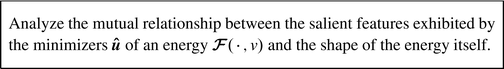
This problem was posed in a systematic way and studied since [74, 75]. The point of view provided by (7) is actually adopted by many authors. Problem (7) is totally general and involves crucial stakes:
of obeys all information contained in the data model as well as in the prior . Hence the question: how the prior and the data-fidelity are effectively involved in – a minimizer of . This leads to formulate the following inverse modeling problem:(7)
It yields rigorous and strong results on the minimizers .
.
Such a knowledge enables a real control on the solution – the reconstructed image or signal .
.
Conversely, it opens new perspectives for modeling.
It enables the conception of specialized energies that fulfill the requirements in applications.
This kind of results can help to derive numerical schemes using knowledge on the solutions.
Problem (7) remains open. The results presented here concern images, signals, and data living on finite grids. In this practical framework, the results in this chapter are quite general since they hold for energies  which can be convex or nonconvex or smooth or nonsmooth, and results address local and global minimizers.
which can be convex or nonconvex or smooth or nonsmooth, and results address local and global minimizers.Organization of the Chapter
Some preliminary notions and results that help the reading of the chapter are sketched in Sect. 2. Section 3 is devoted to the regularity of the (local) minimizers of  with a special focus on nonconvex regularization. Section 4 shows how edges are enhanced using nonconvex regularization. In Sect. 5 it is shown that nonsmooth regularization leads typically to minimizers that are sparse in the space spanned by {D i }. Conversely, Sect. 6 exhibits that the minimizers relevant to nonsmooth data fidelity achieve an exact fit for numerous data samples. Section 7 considers results when both
  and
and  are nonsmooth. Illustrations and applications are presented.
with a special focus on nonconvex regularization. Section 4 shows how edges are enhanced using nonconvex regularization. In Sect. 5 it is shown that nonsmooth regularization leads typically to minimizers that are sparse in the space spanned by {D i }. Conversely, Sect. 6 exhibits that the minimizers relevant to nonsmooth data fidelity achieve an exact fit for numerous data samples. Section 7 considers results when both and are nonsmooth. Illustrations and applications are presented.2 Preliminaries
In this section we set the notations and recall some classical definitions and results on minimization problems.
Notation
We systematically denote by  a (local) minimizer of
  . It is explicitly specified when
  is a global minimizer.
a (local) minimizer of . It is explicitly specified when is a global minimizer.
D j n – The differential operator of order n with respect to the jth component of a function.
v[i] – The ith entry of vector v.
# J – The cardinality of the set J.
J c = I∖J – The complement of J ⊂ I in I where I is a set.
 – The orthogonal complement of a sub-vector space
  .
.
A ∗ – The transpose of a matrix (or a vector) where A is real valued.
 (
( ) – The matrix A is positive definite (positive semi-definite)
 –The n-length vector composed of ones, i.e.,
 ![$$\mathbb{1}_{n}[i] = 1$$](/wp-content/uploads/2016/04/A183156_2_En_5_Chapter_IEq82.gif) ,
,  .
.
 – The Lebesgue measure on
  .
.
 – The identity operator.
 – A vector or a matrix ρ-norm.
 and
and , i.e., e i [i] = 1 and e i [j] = 0 if i ≠ j.
Reminders and Definitions
Definition 1.
A function  is coercive if
  .
.
is coercive if .A special attention being dedicated to nonsmooth functions, we recall some basic facts.
Definition 2.
Given  , the function
  admits at
  a one-sided derivative in a direction
  , denoted
  , if the following limit exists:
 where the index 1 in δ 1 means that derivatives with respect to the first variable of
  are addressed.
, the function admits at a one-sided derivative in a direction , denoted , if the following limit exists: are addressed.Here  is a right-side derivative; the left-side derivative is
  . If
. If  is differentiable at
  , then
  where D 1 stands for differential with respect to the first variable (see paragraph “Notation”). For
  , we denote by ϕ′(t −) and ϕ′(t +) its left-side and right-side derivatives, respectively.
is a right-side derivative; the left-side derivative is . If is differentiable at , then where D 1 stands for differential with respect to the first variable (see paragraph “Notation”). For , we denote by ϕ′(t −) and ϕ′(t +) its left-side and right-side derivatives, respectively.The classical necessary condition for a local minimum of a (nonsmooth) function is recalled [60, 86]:
Theorem 1.
If  has a local minimum at
  , then
  , for every
  .
.
has a local minimum at , then , for every .If  is Fréchet differentiable at
  , one finds
  .
.
is Fréchet differentiable at , one finds .Rademacher’s theorem states that if  is proper and Lipschitz continuous on
  , then the set of points in
  at which
  is not Fréchet differentiable form a set of Lebesgue measure zero [60, 86]. Hence
  is differentiable at almost every u. However, when
  is nondifferentiable, its minimizers are typically located at points where
  is nondifferentiable; see, e.g., Example 1 below.
is proper and Lipschitz continuous on , then the set of points in at which is not Fréchet differentiable form a set of Lebesgue measure zero [60, 86]. Hence is differentiable at almost every u. However, when is nondifferentiable, its minimizers are typically located at points where is nondifferentiable; see, e.g., Example 1 below.Example 1.
Consider  for β > 0 and
  . The minimizer
  of
of  reads as
![$$\displaystyle{\hat{u} = \left \{\begin{array}{ccc} 0 &\mbox{ if}& \vert v\vert \leqslant \beta \\ v -\mathrm{ sign }(v)\beta &\mbox{ if} &\vert v\vert >\beta \end{array} \right.\ \ \ \ \ \mbox{ $\mathsf{(\hat{u}isshrunkw.r.t.v.)}$}}$$” src=”/wp-content/uploads/2016/04/A183156_2_En_5_Chapter_Equd.gif”></DIV></DIV></DIV>Clearly, <SPAN id=IEq123 class=InlineEquation><IMG alt=$$\mathcal{F}(\cdot,v)$$ src=]() is not Fréchet differentiable only at zero. For any
is not Fréchet differentiable only at zero. For any  , the minimizer of
  is located precisely at zero.
for β > 0 and . The minimizer of reads as, the minimizer of is located precisely at zero. The next corollary shows what can happen if the necessary condition in Theorem 1 fails.
Corollary 1.
Let  be differentiable on
  where
where
 , if
, if  is a (local) minimizer of
  then
then

 .
.
 .
.
Get Clinical Tree app for offline access

be differentiable on where, if is a (local) minimizer of thenProof.


Example 2.
Suppose that  in (3) is a differentiable function for any
  . For a finite set of positive numbers, say θ 1, …, θ k , suppose that the PF ϕ is differentiable on
  and that
![$$\displaystyle{ \phi '\left (\theta _{j}^{-}\right ) >\phi ‘\left (\theta _{ j}^{+}\right ),\quad 1\leqslant j\leqslant k. }$$” src=”/wp-content/uploads/2016/04/A183156_2_En_5_Chapter_Equ10.gif”></DIV></DIV><br />
<DIV class=EquationNumber>(10)</DIV></DIV>Given a (local) minimizer <SPAN id=IEq137 class=InlineEquation><IMG alt=$$\hat{u}$$ src=]() , denote
, denote
 Define
  , which is differentiable at
  . Clearly,
  . Applying the necessary condition (9) for
  yields
 In particular, one has
  , which contradicts the assumption on ϕ′ in (10). It follows that if
  is a (local) minimizer of
  , then
  and
and
 A typical case is the PF (f6) in Table 1, namely, ϕ(t) = min{α t 2, 1}. Then k = 1 and
  .
.
in (3) is a differentiable function for any . For a finite set of positive numbers, say θ 1, …, θ k , suppose that the PF ϕ is differentiable on and that, which is differentiable at . Clearly, . Applying the necessary condition (9) for yields, which contradicts the assumption on ϕ′ in (10). It follows that if is a (local) minimizer of , then and.The following existence theorem can be found, e.g., in the textbook [35].
Theorem 2.
For  , let
, let  be a nonempty and closed subset and
  a lower semicontinuous (l.s.c.) proper function. If U is unbounded (with possibly
  ), suppose that
  is coercive. Then there exists
  such that
  .
.
, let be a nonempty and closed subset and a lower semicontinuous (l.s.c.) proper function. If U is unbounded (with possibly ), suppose that is coercive. Then there exists such that .This theorem gives only sufficient conditions for the existence of a minimizer. They are not necessary, as seen in the example below.
Example 3.
Let  involve (f6) in Table 1 and read
![$$\displaystyle{\mathcal{F}(u,v) = (u[1] - v[1])^{2} +\beta \phi (\vert \,u[1] - u[2]\,\vert )\ \ \ \mbox{ for}\ \ \ \phi (t) =\max \{\alpha t^{2},1\},\ \ \ 0 <\beta < \infty.}$$](/wp-content/uploads/2016/04/A183156_2_En_5_Chapter_Equi.gif) For any v,
For any v,  is not coercive since it is bounded by β in the direction spanned by
 ![$$\left \{(0,u[2])\right \}$$](/wp-content/uploads/2016/04/A183156_2_En_5_Chapter_IEq156.gif) . However, its global minimum is strict and is reached for
. However, its global minimum is strict and is reached for ![$$\hat{u}[1] =\hat{ u}[2] = v[1]$$](/wp-content/uploads/2016/04/A183156_2_En_5_Chapter_IEq157.gif) with
with  .
.
involve (f6) in Table 1 and read is not coercive since it is bounded by β in the direction spanned by . However, its global minimum is strict and is reached for with .To prove the existence of optimal solutions for more general energies, we refer to the textbook [9].
Most of the results summarized in this chapter exhibit the behavior of the minimizer points  of
of  under variations of v. In words, they deal with local minimizer functions.
of under variations of v. In words, they deal with local minimizer functions.Definition 3.
Let  and
and  . We say that
  is a local minimizer function for the family of functions
  if for any v ∈ O, the function
  reaches a strict local minimum at
  .
.
and . We say that is a local minimizer function for the family of functions if for any v ∈ O, the function reaches a strict local minimum at .
Theorem 3.
Let  be proper, convex, l.s.c., and coercive for every
  .
.
be proper, convex, l.s.c., and coercive for every .(i)
Then  has a unique (global) minimum which is reached for a closed convex set of minimizers
  .
.
has a unique (global) minimum which is reached for a closed convex set of minimizers .(ii)
If in addition  is strictly convex, then there is a unique minimizer
  (which is also global). So
  has a unique minimizer function
  .
.
is strictly convex, then there is a unique minimizer (which is also global). So has a unique minimizer function .The next lemma, which can be found, e.g., in [52], addresses the regularity of the local minimizer functions when  is smooth. It can be seen as a variant of the implicit functions theorem.
is smooth. It can be seen as a variant of the implicit functions theorem.Lemma 1.
Let  be
be  ,
,  , on a neighborhood of
  . Suppose that
  reaches at
  a local minimum such that
  . Then there are a neighborhood
  containing v and a unique
  local minimizer function
  , such that
  for every ν ∈ O and
  .
.
be , , on a neighborhood of . Suppose that reaches at a local minimum such that . Then there are a neighborhood containing v and a unique local minimizer function , such that for every ν ∈ O and .This lemma is extended in several directions in this chapter.
Definition 4.
Let  and
and  an integer. We say that ϕ is
  on
on  , or equivalently that
  , if and only if
  is
is  on
on  .
.
and an integer. We say that ϕ is on , or equivalently that , if and only if is on .By this definition, ϕ′(0) = 0. In Table 1, left,  for (f1) if α < 2,
  for (f4), while for (f2), (f3), and (f7)–(f9) we find
  .
.
for (f1) if α < 2, for (f4), while for (f2), (f3), and (f7)–(f9) we find .3 Regularity Results
Here, we focus on the regularity of the minimizers of  of the form
where  and for any i ∈ I we have
  for
for  . Let us denote by D the following rs × p matrix:
![$$\displaystyle{\mathrm{D}\stackrel{\mathrm{def}}{=}\left [\begin{array}{@{}c@{}} \mathrm{D}_{1}\\ \ldots \\ {\mathrm{D}_{r}} \end{array} \right ].}$$](/wp-content/uploads/2016/04/A183156_2_En_5_Chapter_Equj.gif) When A in (11) is not injective, a standard assumption in order to have regularization is
When A in (11) is not injective, a standard assumption in order to have regularization is
of the form(11)
and for any i ∈ I we have for . Let us denote by D the following rs × p matrix:H3
.

Some General Results
We first verify the conditions on  in (11) that enable Theorems 2 and 3 to be applied. Since H1 holds,
  in ( 11 ) is l.s.c. and proper.
in (11) that enable Theorems 2 and 3 to be applied. Since H1 holds, in ( 11 ) is l.s.c. and proper.


However, the PFs involved in (11) used for signal and image processing are often nonconvex, bounded, or nondifferentiable. One extension of the standard results is given in the next section.
Stability of the Minimizers of Energies with Possibly Nonconvex Priors
Related questions have been considered in critical point theory, sometimes in semi-definite programming; the well-posedness of some classes of smooth optimization problems was addressed in [42]. Other results have been established on the stability of the local minimizers of general smooth energies [52]. Typically, these results are quite abstract to be applied directly to energies of the form (11).
Here the assumptions stated below are considered.


Under H1, H2, H4, and H5, the prior  (and hence
  ) in (11) can be nonconvex and in addition nonsmooth. By H1 and H4,
  in (11) admits a global minimum
  – see Item 1 in section “Some General Results.” However,
  can present numerous local minima.
(and hence ) in (11) can be nonconvex and in addition nonsmooth. By H1 and H4, in (11) admits a global minimum – see Item 1 in section “Some General Results.” However, can present numerous local minima.
Energies with nonconvex and possibly nondifferentiable PFs ϕ are frequently used in engineering problems since they were observed to give rise to high-quality solutions
  . It is hence important to have good knowledge on the stability of the obtained solutions.
The results summarized in this section provide the state of the art for energies of the form (11).
Local Minimizers
The stability of local minimizers is an important matter in its own right for several reasons. Often, a nonconvex energy is minimized only locally, in the vicinity of some initial guess. Second, the minimization schemes that guarantee the finding of the global minimum of a nonconvex objective function are exceptional. The practically obtained solutions are usually only local minimizers.
The statements below are a simplified version of the results established in [44].
Theorem 4.


Since  is closed in
  and
and  , the stated properties are generic.
is closed in and , the stated properties are generic.Commentary on the Assumptions
All assumptions H1, H2, and H5 bearing on the PF ϕ are nonrestrictive; they address all PFs in Table 1 except for (f13) which is discontinuous at zero. The assumption H4 cannot be avoided, as seen in Example 4.
Example 4.
Consider  given by
![$$\displaystyle{\mathcal{F}(u,v) = \left (u[1] - u[2] - v\right )^{2} + \vert u[1]\vert + \vert u[2]\vert,}$$](/wp-content/uploads/2016/04/A183156_2_En_5_Chapter_Equk.gif) where
where ![$$v \equiv v[1]$$](/wp-content/uploads/2016/04/A183156_2_En_5_Chapter_IEq250.gif) . The minimum is obtained after a simple computation.
. The minimum is obtained after a simple computation.
![$$\displaystyle\begin{array}{rcl} v > \frac{1} {2}\quad & & \hat{u} = \left (c,c – v + \frac{1} {2}\right )\ \ \mbox{ for any}\ \ c \in \left [0,v -\frac{1} {2}\right ]\ \ \ \mbox{ (nonstrict minimizer)}. {}\\ \vert v\vert \leq \frac{1} {2}\quad & & \hat{u} = 0\ \ \ \mbox{ (unique minimizer)} {}\\ v < -\frac{1} {2}\quad & & \hat{u} = \left (c,c - v -\frac{1} {2}\right )\ \ \mbox{ for any}\ \ c \in \left [v + \frac{1} {2},0\right ]\ \ \ \mbox{ (nonstrict minimizer)}. {}\\ \end{array}$$](/wp-content/uploads/2016/04/A183156_2_En_5_Chapter_Equ12.gif) In this case, assumption H4 fails and there is a local minimizer function only for
In this case, assumption H4 fails and there is a local minimizer function only for ![$$v \in \left [-\frac{1} {2}, \frac{1} {2}\right ]$$](/wp-content/uploads/2016/04/A183156_2_En_5_Chapter_IEq251.gif) .
.
given by. The minimum is obtained after a simple computation..Other Results
The derivations in [44] reveal several other practical results.
1.
If  , see Definition 4, then
  , every local minimizer
  of
of  is strict and
  . Consequently, Lemma 1 is extended since the statement holds true
  .
.
, see Definition 4, then , every local minimizer of is strict and . Consequently, Lemma 1 is extended since the statement holds true .
For real data v – a random sample of – whenever
  is differentiable and satisfies the assumptions of Theorem 4 , it is a generic property that local minimizers
  are strict and their Hessians
  are positive definite.

3.
If ϕ′(0+) > 0, define
Then  , every local minimizer
  of
of  is strict and
(12)
, every local minimizer of is strict and(a)
 – a sufficient condition for a strict minimum on
  .
.
– a sufficient condition for a strict minimum on .(b)
 .
.
.


Global Minimizers of Energies with for Possibly Nonconvex Priors
Theorem 5.


Otherwise said, in a real-world problem there is no chance of getting data v such that the energy (11) has more than one global minimizer.
Nonetheless,  plays a crucial role for the recovery of edges; this issue is developed in Sect. 4.
plays a crucial role for the recovery of edges; this issue is developed in Sect. 4.Nonasymptotic Bounds on Minimizers
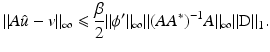
The aim here is to give nonasymptotic analytical bounds on the local and the global minimizers  of
of  in (11) that hold for all PFs ϕ in Table 1. Related questions have mainly been considered in particular cases or asymptotically; see, e.g., [4, 71, 92]. In [51] the mean and the variance of the minimizers
  for strictly convex and differentiable functions ϕ have been explored.
of in (11) that hold for all PFs ϕ in Table 1. Related questions have mainly been considered in particular cases or asymptotically; see, e.g., [4, 71, 92]. In [51] the mean and the variance of the minimizers for strictly convex and differentiable functions ϕ have been explored.The bounds provided below are of practical interest for the initialization and the convergence analysis of numerical schemes. The statements given below are extracted from [82].
Bounds on the restored data.
One compares the “restored” data  with the given data v.
with the given data v.H6
Consider the alternative assumptions:
 and
and  where the set
 on
 .
.
The set  allows us to address the PF given in (f6). Let us emphasize that under H1 and H6, the PF ϕ can be convex or nonconvex.
allows us to address the PF given in (f6). Let us emphasize that under H1 and H6, the PF ϕ can be convex or nonconvex.Theorem 6.


Comments on the results.
This bound holds for every (local) minimizer of  . If A is a uniform tight frame (i.e., A ∗ A = Id), one has

. If A is a uniform tight frame (i.e., A ∗ A = Id), one hasThe mean of restored data.
In many applications, the noise corrupting the data can be supposed to have a mean equal to zero. When A = Id, it is well known that mean mean(v); see, e.g., [7]. However, for a general A one has
The requirement  is quite restrictive. In the simple case when ϕ(t) = t 2,
  and A is square and invertible, it is easy to see that this is also a sufficient condition. Finally, if
  , then generally mean
  mean
mean  .
.
mean(v); see, e.g., [7]. However, for a general A one has(13)
is quite restrictive. In the simple case when ϕ(t) = t 2, and A is square and invertible, it is easy to see that this is also a sufficient condition. Finally, if , then generally mean mean .The residuals for edge-preserving regularization.
A bound on the data-fidelity term at a (local) minimizer  of
of  shall be given. The edge-preserving H2 (see Sect. 1) is replaced by a stronger edge-preserving assumption:
of shall be given. The edge-preserving H2 (see Sect. 1) is replaced by a stronger edge-preserving assumption:H7
.Except for (f1) and (f13), all other PFs in Table 1 satisfy H7. Note that when ϕ′(0+) > 0 and H7 hold, one usually has  .
.
.Theorem 7.


Let us emphasize that the bound in (14) is independent of data v and that it is satisfied for any local or global minimizer  of
of  . (Recall that for a real matrix C with entries C[i, j], one has
 ![$$\|C\|_{1} =\max _{j}\sum _{i}\vert C[i,j]\vert $$](/wp-content/uploads/2016/04/A183156_2_En_5_Chapter_IEq328.gif) and
and ![$$\|C\|_{\infty } =\max _{i}\sum _{j}\vert C[i,j]\vert $$](/wp-content/uploads/2016/04/A183156_2_En_5_Chapter_IEq329.gif) ; see, e.g., [35].)
; see, e.g., [35].)
of . (Recall that for a real matrix C with entries C[i, j], one has and ; see, e.g., [35].)If  corresponds to a discrete gradient operator for a two-dimensional image,
  . If in addition A = Id, (14) yields
corresponds to a discrete gradient operator for a two-dimensional image, . If in addition A = Id, (14) yieldsThe result of this theorem may seem surprising. In a statistical setting, the quadratic data-fidelity term  in (11) corresponds to white Gaussian noise on the data, which is unbounded. However, if ϕ is edge preserving according to H7, any (local) minimizer
  of
of  gives rise to a noise estimate
 ![$$(v - A\hat{u})[i]$$](/wp-content/uploads/2016/04/A183156_2_En_5_Chapter_IEq335.gif) ,
,  that is tightly bounded as stated in (14).
in (11) corresponds to white Gaussian noise on the data, which is unbounded. However, if ϕ is edge preserving according to H7, any (local) minimizer of gives rise to a noise estimate , that is tightly bounded as stated in (14).
Hence the model for Gaussian noise on the data v is distorted by the solution .
.
When is convex and coercive
Related posts:
 Segmentation with Shape Priors: Explicit Versus Implicit Representations
 Transform in Astronomical Data Processing
 Methods for Multi-dimensional Visual Data Analysis
 Set Methods for Structural Inversion and Image Reconstruction
 Methods for Ill-Posed Problems
 and Shah Model and Its Applications to Image Segmentation and Image Restoration

Stay updated, free articles. Join our Telegram channel

Full access? Get Clinical Tree

