MR Angiography: Techniques and Clinical Applications
Wende N. Gibbs
Joseph E. Heiserman
Introduction
Flow-related phenomena were recognized early in the development of MR (1), well before imaging techniques were devised. Understanding the mechanisms of flow sensitivity and the appearance of flowing fluid is important for several reasons. First, the flow sensitivity can be exploited to provide diagnostic information. Since the initial publication by Wedeen et al. (2) showing intravascular flow as high signal intensity on in vivo MR images, intense scientific and clinical interest has focused on the development of MR angiography (MRA) and its applications to imaging cerebral vasculature and its pathology. Initially, two families of techniques, time of flight (TOF) and phase contrast (3,4), were developed. These rely on the inherent properties of blood and its motion. More recently, rapid acquisition three-dimensional (3D) imaging in combination with T1-shortening intravenous contrast agents was introduced (5). A foundation in the fundamental physical origins of these methods can aid in the interpretation and rational choice among these techniques and their many permutations.
Second, the characteristics of the nuclear magnetic resonance (NMR) signal of flow can be quite variable, even in normal physiologic states. This can have a direct impact on the image appearance of flowing blood; the possibility of misinterpreting normal states as important pathologic conditions is reduced if one has a good understanding of the physical basis of flow effects. It is critically important that interpretation of MR-based flow studies is made with the fundamental understanding that these images depict the physiology of flow, rather than the morphology of the vessel lumen. This is very different from other radiologic methods, like CT angiography (CTA) or catheter angiography, which directly demonstrate the morphology of the patent lumen of a vessel by filling it with a contrast agent.
Third, the variable signal often generates significant artifacts that can obscure anatomy and degrade images. An understanding of flow phenomena allows one to recognize these artifacts and alter protocols to eliminate or compensate for such effects.
Fluid Flow, the Basics
Start by considering the simplest case, an incompressible fluid without viscosity in a rigid circular pipe of constant size. This is known as an ideal or Euler fluid. For slow flow of a fluid approaching this limit, the motion is en masse down the pipe, a condition known as plug flow. Every small volume within the fluid moves at the same velocity. If now the diameter of the pipe changes, the speed of the flow needs to change in proportion to the change in cross-sectional area to ensure continuity of the fluid. This means that to keep the volume flow rate of fluid constant the velocity ν of the fluid must change in proportion to the radius r of the pipe squared,
We can also make a statement about conservation of energy for the flow, known as Bernoulli’s principle. In simplest form, the sum of the pressure p and kinetic energy per unit volume of the flow must be conserved:
where ρ is the density of the fluid.
To get a more realistic picture, add viscosity. Now we think of the flowing fluid as being composed of thin concentric circular sheets or laminae. The viscosity results in drag between these sheets, and between the outermost sheet and the wall. Again consider slow flow, let the drag force be proportional to the velocity, and let the velocity at the wall be zero. This is known as a Newtonian fluid. In this model, the fluid velocity decreases due to drag as we move from the center of the pipe out toward the wall. It turns out this results in a parabolic flow profile, known as laminar flow (Fig. 25.1). Because of the reduction in velocity peripherally,
the volume flow rate Q is reduced, especially in smaller pipes, and depends on the fourth power of the radius. This is known as Poiseuille flow,
the volume flow rate Q is reduced, especially in smaller pipes, and depends on the fourth power of the radius. This is known as Poiseuille flow,
 FIGURE 25.1 In well-ordered laminar flow, the velocity is constant on sets of shells or “laminae.” Because of friction due to viscosity between the fluid and the wall, the fluid velocity at the wall is zero. In a long cylindrical tube with rigid walls, the laminae are concentric cylinders. With steady flow, the velocity profile across the tube is parabolic, as shown by the dashed line. This case (steady flow in a long, rigid-walled, cylindrical vessel) is referred to as Poiseuille flow. |
Because of this strong dependence on radius, changes in the vessel size in the vascular tree can effectively control flow.
Next consider a smooth bend in the pipe. In steady flow, the fluid parcels resist the change in direction due to inertia. When centrifugal forces are large compared to viscous damping, this leads to a spiral motion of the fluid around the bend. In addition, slower moving peripheral fluid parcels are more easily accelerated, causing a more pluglike profile to develop. Even in relatively simple geometries, flow patterns can become complex. This is illustrated for the carotid bifurcation in Figure 25.2.
In vivo vascular flow is associated with additional complexity. Arteries and veins are not rigid uniform pipes but are elastic with varying diameter and numerous branchings. In vivo flow is also pulsatile, and this is associated with variation of flow velocity with time and even at different points within vessels. When the unsteady forces associated with acceleration of flow are large compared to viscous damping, pulsatile flow will tend to be associated with a flatter, nonlaminar flow profile. Blood is not well modeled as a Newtonian fluid in smaller vessels because the cellular components lead to vessel diameter–dependent viscous forces. Because of these and other factors, in vivo flow is frequently not well modeled by a laminar profile, and may be complex and disordered, especially in the presence of pathology. As an example, Figure 25.3 shows flow patterns associated with an experimental stenosis. When flow becomes so complex that the flow velocity at any given point is random, the pattern is referred to as turbulent. In this case the viscous forces within the fluid are too small to damp the inertial motions of the fluid. This rarely occurs in the vascular system, even in high-flow regions distal to stenoses. However, flow within the vascular tree can become sufficiently disordered that even at a very small scale the direction of flow can vary from point to point.
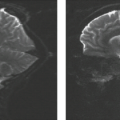
 FIGURE 25.2 Flow patterns as shown by particle trajectories. These were measured with high-speed photography through a constant-flow phantom fashioned from cadaver specimens of the human carotid artery bifurcation. Re0 is a measure of the ratio of fluid inertia to viscous drag known as the Reynolds number, U0 is the average velocity, Q0, Q1, and Q2 are the flows in the common internal and external carotid arteries, respectively. Overlay numbers in the top illustration are the local flow velocity values. In the lower illustration, numbers within the flow channel show the peak velocity at a number of cross-sectional positions, and the values at the edge of the vessel are the local shear rate. (From Motomiya M, Karino T. Flow patterns in the human carotid artery bifurcation. Stroke 1984;15:50–56, with permission.) |
 FIGURE 25.3 Visualization of the flow field through a 50% (by area) axisymmetric stenosis. The stenosis is visible at the left of each tube. The flow rate was temporally steady from left to right. Three flow conditions are shown, with flow velocity increasing from frame A to C. Visualization was performed by injecting hydrogen bubbles into the flowing fluid (63% by weight glycerol in water), illuminating the system with four lamps, and using optical photography. Note that at higher velocities the flow becomes quite complex. (From Ahmed SA, Giddens DP. Velocity measurements in steady flow through axisymmetric stenoses at moderate Reynolds numbers. J Biomech 1983;16:505–516, with permission.) |
These simple models will provide sufficient framework for the understanding of most MR flow phenomena; however, the interested reader is referred to the literature for a more detailed picture of blood flow (6).
Effects of Motion on MR
Broadly speaking, motion may affect an MR signal by modifying its amplitude or its phase. A change in amplitude related to fluid motion is referred to as a TOF effect. Changes in phase are discussed in a later section.
Time of Flight
TOF effects arise due to the macroscopic motion of spins and their state of longitudinal magnetization. Typically, the magnetization of a bolus of blood is modified (with a radiofrequency [RF] pulse) at one location and detected at another. If the direction of flow is perpendicular to the imaging slice (or volume), partially saturated spins are replaced by the inflowing unsaturated (fully relaxed and magnetized) spins during the RF repetition time (TR). The degree of replacement of partially saturated spins is directly dependent on the flow velocity and slice thickness (Fig. 25.4). If the TR is short relative to the longitudinal relaxation time T1 of stationary tissue, the signal of the stationary material is saturated and therefore signal from this source is attenuated. Signal from the unsaturated inflowing blood entering the excitation volume between pulse sequence repetitions consequently has a high signal intensity compared to the surrounding stationary tissue. This is flow-related enhancement.
In the simplest example, consider a volume of tissue being imaged using a pulse sequence with TR less than the T1 of blood. Assume for now that during the TR interval there is no RF excitation outside of the imaged volume (e.g., we are using a 3D sequence or a single-slice 2D sequence). We also assume that the transverse magnetization at the end of each TR is zero (e.g., because TR is significantly longer than T2). Static tissue, including static blood, will experience a long train of excitations (one per sequence repetition) and reach a steady-state signal that depends on parameters such as TR, flip angle, and echo
time (TE). Because TR is less than T1, the magnetization of static spins will be partly saturated. Flowing spins, however, if flowing sufficiently rapidly, will not have seen the long train of excitations and therefore will be more fully magnetized. The signal from flowing fluid will depend on the sequence parameters but also on the amount of spin replacement.
time (TE). Because TR is less than T1, the magnetization of static spins will be partly saturated. Flowing spins, however, if flowing sufficiently rapidly, will not have seen the long train of excitations and therefore will be more fully magnetized. The signal from flowing fluid will depend on the sequence parameters but also on the amount of spin replacement.
 FIGURE 25.4 Illustration of flow-related enhancement. The schematic shows the cross section of a vessel. The relaxed spins entering the image slice result in high signal intensity because of the inflow of fully magnetized blood into the excitation volume. Signal strength is proportional to the fractional replacement of saturated spins within the imaging volume. |
The effect is the simplest if the excitation is with 90-degree pulses. Any intravascular volume element (voxel) will contain a mixture of two subpopulations, fully magnetized spins that are experiencing their first excitation and spins that have been previously excited. For a velocity ν in the slice direction and a slice thickness of Δz, the fraction of fully magnetized spins is νTR/Δz (but no greater than 1). Therefore, as a function of ν, the signal intensity will increase linearly until it plateaus at a velocity of ν = Δz/TR, where there is full spin replacement and no further signal increase is possible. This signal increase (as compared with that normally expected from the NMR properties of the fluid) represents flow-related enhancement. Note that for typical flow profiles in which the velocity is not uniform across the diameter, the flow-related enhancement is nonuniform.
The signal behavior of flowing fluid is somewhat more complicated with sequences that use a flip angle other than 90 degrees because the spins do not reach a longitudinal steady state after only one TR. For a given flow velocity, a voxel will contain some spins that are about to experience their first excitation, some that will see their second, and so on. For example, spins moving at 15 cm/s into the imaging volume travel 4.5 mm in a TR of 30 ms. With a 10-mm slice, there would be 45% (4.5/10) spin replacement per TR. Just before any RF pulse, therefore, 45% of the spins are fully magnetized, 45% have experienced one RF pulse, and 10% (the remainder) have experienced two RF pulses.
The contrast (i.e., signal difference) between flowing blood and surrounding tissue depends on the signal behavior of the blood but is further affected by saturation of the magnetization of static spins. Higher flip angles and shorter TRs lead to more saturation and lower signal from static tissue and therefore higher contrast. As a result, maximum contrast is obtained at higher flip angles than predicted by the intravascular signal alone.
In volumetric imaging, flow-related enhancement is stronger at the ends of the imaging volume. Well within the imaging volume, spins are likely to have been partly saturated by earlier excitation pulses. It should be kept in mind that this “entry slice” phenomenon occurs only for surfaces defined by selective excitation pulses (e.g., in the slice or slab direction). It will not be seen at the edges of the volume in the readout or phase-encoded directions. For any vessel, signal increases will be highest near the surface where that vessel enters the excitation volume.
Pulsatile Flow
A priori, we might assume that the average velocity determines the overall signal intensity changes from TOF effects. However in very short TR sequences, contrast in the image might be determined by data collected during a fraction of the cardiac cycle, and as a result, the image intensity may be dominated by the flow conditions during that fraction of the cycle. This can lead to different intravascular signal intensities in different images if they are not consistently synchronized to the cardiac cycle. In 2D TOF MRA, this can lead to inconsistent vessel intensity, which may be especially troublesome in computed projections. Synchronization between physiologic periodicity and signal acquisition may also undermine the assumption that the image intensity should reflect the average flow velocity. This synchronization may be accidental or intentional. For example, when the cardiac cycle has a period close to the TR (known as pseudogating), one slice in an interleaved multislice scan may be acquired predominantly during systole and another predominantly during diastole. This is more pronounced with intentional synchronization to the cardiac cycle (i.e., cardiac triggering).
Tagging, Suppression, and Labeling Pulses
Flow-related enhancement is caused by the inflow of fully magnetized spins into the imaging volume. A number of techniques deliberately alter the longitudinal magnetization of spins outside the imaging volume to affect their appearance when they are in the volume of interest. Saturation pulses can be selectively applied upstream from the imaged volume to reduce the longitudinal magnetization of fluid that will flow into the volume. To be effective, the presaturation pulses need to be applied frequently and/or in close temporal proximity to the slice excitation. In 2D TOF, this can be done by placing the saturation pulse always immediately adjacent to the slice being collected, this is known as a traveling presaturation pulse. In 3D TOF, the impact may be most visible in the entry slices.
Phase Effects
After a 90-degree pulse, the magnetization vector lies in the transverse plane and precesses at the local Larmor frequency. The phase of the MR signal can be visualized as the position of the transverse magnetization vector relative to some standard. A useful analogy is the position of the hand of a clock relative to the 12 o’clock position. Another class of flow effects results from changes in the phase of the transverse magnetization that occur when spins move along magnetic field gradients such as those used for position encoding in MR. This arises from local changes in the Larmor frequency due to the presence of the gradient. Moving spins change location during gradient play and as a consequence of this motion within the gradient field acquire additional phase changes. Consider first a stationary spin at position x0 subjected to a gradient of constant amplitude G and duration δ (Fig. 25.5A). The phase change φ due to the presence of the gradient magnetic field is given by
where γ is a constant known as the gyromagnetic ratio and x0 is the position of the stationary spin. For this simple case of
a gradient of constant amplitude, the phase change is proportional to the factor Gδ which represents the “area” of the gradient play and is referred to as the zeroth moment. Consider now the case of motion. For a spin moving at constant speed ν in the x direction, there is an additional velocity-related contribution to the phase, and the total change can be written as
a gradient of constant amplitude, the phase change is proportional to the factor Gδ which represents the “area” of the gradient play and is referred to as the zeroth moment. Consider now the case of motion. For a spin moving at constant speed ν in the x direction, there is an additional velocity-related contribution to the phase, and the total change can be written as
where T is the time between the excitation pulse and the center of the readout pulse. The factor GδT is referred to as the first moment.
 FIGURE 25.5 Three gradient waveforms used to explain motion-induced phase shifts (see text): (A) a phase-encoding gradient of amplitude G and duration δ centered at time T after the excitation pulse, (B) a bipolar lobe composed of two pulses of duration δ and center-to-center spacing Δ but opposite amplitudes ±G, and (C) a waveform with a first moment of zero. |
Consider now a more complex gradient with a negative going component (lobe) of duration δ followed by a positive lobe of equal amplitude and duration, with a center-to-center spacing of Δ (Fig. 25.5B). This is known as a bipolar gradient pair. Because the two lobes have equal but opposite area, the net area is effectively zero. Because the (position-dependent) phase change introduced by the first lobe is cancelled by the second lobe of identical size and duration but opposite polarity, the zeroth moment is zero and stationary spins experience a net phase change of zero. However, the contribution from the moving spins is nonzero, and the phase change for times after the end of the bipolar gradient (and for constant-velocity motion) becomes
An intuitive way to interpret this is as follows. The first lobe imposes a phase shift of (−γGδ) on the spins at the time of the center of this first lobe. The second lobe imposes an additional phase shift of (+γGδ) times the position of the spins at the time of the center of the second lobe. The net effect is a phase shift of (γGδ) times the distance the spins traveled during the time between the center of one lobe and the center of the other. With constant-velocity motion, this displacement is νΔ, making the net phase shift (γGδ)(νΔ).
Bipolar gradients can be used to reduce the velocity sensitivity (or even set it to zero). In Figure 23.5C, a bipolar lobe (filled in with the diagonal pattern) is preceded by a bipolar lobe of opposite amplitude. The two act on the spins in succession. The first (filled in with the dotted pattern) introduces a phase shift proportional to velocity. The second bipolar lobe (filled in with the diagonal pattern) introduces an opposing velocity-induced phase shift. As a whole, this waveform has a first moment of zero and therefore no velocity sensitivity. The dotted pattern lobe was used to alter the velocity sensitivity that would have been present had the second lobe been used by itself. This approach is used to alter the velocity sensitivity of pulse sequences, for example, in gradient moment nulling.
Although the waveform of Figure 25.5C is insensitive to velocity (because it has a zero first moment), it is sensitive to acceleration. This sensitivity can be understood, as before, by realizing that the first part of the waveform introduces a phase shift dependent on the velocity at one time point (the center of the first bipolar lobe), whereas the second portion removes a phase shift depending on the velocity at the second time point (the center of the second bipolar lobe). If the velocity is the same at the two times, the net phase shift is zero. Otherwise, the net phase shift is proportional to the change in velocity (i.e., the acceleration). Similar considerations apply to even higher-order moments.
Pulse Sequence Considerations
A spin-echo (SE) sequence typically begins with a 90-degree RF pulse followed by a 180-degree refocusing pulse. Both pulses are slice selective. Consequently, flowing blood within the slice during the 90-degree pulse will be labeled, but will have exited the slice and be at a new location during the 180-degree pulse and readout. The blood within the slice at these later times does not contribute signal, and so the vessels appear as signal voids for sufficiently rapid flow. This is referred to as high-velocity signal loss. The TR chosen for an SE sequence must also be long enough to allow the time interval needed for formation of an echo. Gradient-echo (GE) sequences dispense with the 180-degree pulse. The refocusing gradient is nonslice selective, and so even signal from sufficiently rapidly flowing blood is recovered and vessels appear bright, part of the basis of flow-related enhancement. With flip angles less than 90 degrees and short TR, image data can be rapidly acquired. Dephasing of residual transverse magnetization can be accomplished with RF or GE spoiling pulses, resulting in T1-weighted (spoiled gradient-recalled acquisition in the steady state [SPGR], T1-weighted fast field echo [T1 FFE], fast low-angle shot [FLASH]). These benefits are important factors in the choice of GE-based sequences for most angiographic applications.
Flow-Related Artifacts
The basic motion effects (TOF and phase shift effects) can cause increases or decreases in the MR signal amplitude and phase of moving spins. If these signal amplitude changes are consistent throughout the scan, the impact on the image is simply due to the corresponding signal amplitude and/or phase change in intravascular voxels. Consistent flow-related enhancement, for example, causes an increase in intravascular signal in GE images. Consistent phase shifts are harnessed in phase-contrast angiography to depict regions of flow. The most powerful way to ensure that the motion effects are consistent is to ensure that the velocity distributions are temporally steady during the scan time or that the system is synchronized to the variability.
If the signal changes are not consistent throughout the scan, the modulation of the raw data will cause artifacts. Specifically, they will cause some of the signal that actually belongs in one pixel to be dispersed or spread to other image pixels.
Gradient Moment Reduction and Nulling
As has been discussed, motion in the presence of magnetic field gradients causes a phase shift in the transverse magnetization as compared with that of identical static spins at the same location. Through this mechanism, nonuniform velocity within a voxel can lead to nonuniform phase and consequently loss of signal (intravoxel dephasing). If the velocity distribution is not steady in time, ghost artifacts can result due to phase modulation of the average signal from a voxel or from amplitude variations due to time-dependent intravoxel dephasing. Although some of these artifacts are caused by gradients produced by inhomogeneity of the static magnetic field, the strongest effects are due to the magnetic field gradients intentionally applied during the imaging process. The effect of these gradients depends on the details of the waveforms.
A very basic and quite effective method of reducing gradient moments is to reduce the area of the corresponding gradient pulses. There are two important examples of this in MR imaging (MRI)—the use of fractional echoes for frequency encoding in GE imaging and the use of slab excitation and 3D volume imaging rather than acquisition of multiple thin slices. Offsetting the echo within the acquisition window toward the beginning of the readout reduces the area of the dephasing gradient pulse and also allows the time between the center of the dephasing lobe and the center of the echo to be decreased. This technique is also known as “asymmetric” or “partial echo” sampling. The reduction of the first moment can be proportional to the square of the offset, one factor deriving from each of the decrease in area and the decrease in spacing. These design options are often used to obtain a shorter TE, in order to minimize intravoxel dephasing. The improvement is due to both the reduction in gradient moment and TE reduction, but the dominant contribution is the reduction in gradient. The difference between 3D and 2D multislice imaging results from the fact that selective excitation of a thin slice requires very strong gradients. For a constant RF bandwidth, the gradient strength for slice selection is inversely related to slice thickness. Therefore, excitation of a thick slab (for 3D) can be performed with a weaker gradient and a shorter refocusing lobe, both leading to a lower gradient first moment. In addition, 3D images tend to have smaller voxels, leading to less heterogeneity of flow velocities within the voxel and therefore less intravoxel dephasing.
It is also possible to change the gradient moments without altering the spatial encoding lobes. This is generally done by inserting bipolar lobes or by altering the size of other lobes to change the first moment while leaving the net area (zeroth moment) unchanged. Most commercial systems offer first-order gradient moment nulling, a feature that essentially eliminates the phase effects due to constant-velocity motion. Because the first moment is zero, the phase accrual due to the velocity term is zero regardless of the actual velocity. This will greatly decrease intravoxel dephasing, leading to higher signal from flowing spins.
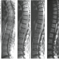
Moment nulling also tends to reduce inconsistencies due to pulsatile flow. Note that first-order moment nulling only eliminates the effect of constant-velocity motion. It may be surprising, then, that it can be effective for pulsatile flow, which by definition exhibits acceleration. However, we need to note that the requirement for first-order nulling to be successful is that the velocity be relatively constant during a single sequence execution. This is easily satisfied, especially for short sequences. Moment nulling reduces the inconsistent phase shift among all the sequence repetitions in the scan from changes in average velocity and thereby leads to artifact reductions (Fig. 25.6).
Imaging Blood Flow
The TOF and phase shift effects discussed previously, although considered primarily in terms of their interference with image interpretation, can be exploited so that both qualitative and quantitative flow information can be extracted from MRI. A
wide variety of techniques can accomplish the general goal of flow detection and blood vessel imaging. Many of the techniques can be divided along the same categories used for discussing basic flow effects: TOF and phase-based methods. In addition, the advent of fast MRI methods has enabled the use of exogenous contrast agents, specifically the arterial phase of the contrast agent transit, to image the vasculature. Some basic aspects of this technique are described in what follows as well.
wide variety of techniques can accomplish the general goal of flow detection and blood vessel imaging. Many of the techniques can be divided along the same categories used for discussing basic flow effects: TOF and phase-based methods. In addition, the advent of fast MRI methods has enabled the use of exogenous contrast agents, specifically the arterial phase of the contrast agent transit, to image the vasculature. Some basic aspects of this technique are described in what follows as well.
 FIGURE 25.6 First-order gradient moment nulling effect on cerebrospinal fluid (CSF) flow. Long–TR/TE image of cervical spine and cord without gradient moment nulling (A) shows signal loss, as well as several ghost images from CSF motion. The artifacts, which degrade the image and obscure the definition of cord from CSF, are virtually eliminated by first-order gradient moment nulling (B), allowing CSF to be seen as high-intensity fluid surrounding the cord. |
Time-of-Flight MR Angiography
By far the most popular TOF MRA methods are based on flow-related enhancement (7). The typical characteristics of these MRA techniques include use of a short TR, partial flip angle GE sequence, coverage of an anatomic volume rather than a single slice, viewing of the data using computed projections, and nonsubtractive imaging, that is, a single acquisition rather than subtraction of two datasets.
In these methods, blood flowing into the region being imaged with the short TR sequence appears as high-contrast “bright blood” signal. The pulse sequence and scanning parameters are selected with consideration given to the expected speed and direction of flow, the vessel tortuosity, and desired field of view (FOV) and spatial resolution. The volumetric acquisition can be executed by sequential scanning of adjacent or even overlapped 2D sections (2D TOF), by imaging the entire volume using a single 3D scan (3D TOF), or by sequential 3D imaging of overlapping slabs. In all three methods, the result is a 3D image array in which, one hopes, the pixels with intravascular blood have the highest signal and the volume is generally viewed using computed projections through the volume.
Two-Dimensional Time of Flight
2D TOF sequences image the 3D volume as a stack of slices that are acquired sequentially (Fig. 25.7). Typically, the orientation of the imaging planes is selected to be perpendicular to the main direction of flow (e.g., axial slices for carotid imaging). Use of thin slices that are relatively perpendicular to the flow produces a high level of spin replacement. In this case a relatively large flip angle yields strong inflow enhancement and good vascular contrast. The amount of spin replacement increases with increasing velocity, increasing TR, and decreasing slice thickness. Without the use of preparation pulses, inflowing blood is bright regardless of flow direction. It is common to use spatial presaturation to select for flow in one direction or the other (i.e., to image arteries vs. veins). Note that this assumes that the flow directions are dependable; errors could be made in regions of retrograde flow. The saturation region is generally moved along with the imaging plane as the multiple slices are sequentially scanned. In all TOF techniques, including 2D TOF, the use of fractional echo methods and a short echo delay (TE) is desirable to minimize phase shifts that can produce regions of signal loss (intravoxel dephasing). The use of first moment nulling is also beneficial even when a penalty in TE is incurred.
 FIGURE 25.7 Sequential two-dimensional time-of-flight technique. Axial gradient-echo images are obtained in a craniocaudad direction with a superiorly placed traveling (tracking) saturation pulse to eliminate inferior flowing venous signal. The direction of acquisition opposing carotid flow minimizes the saturation from a previous slice. |
 FIGURE 25.8 Three-dimensional (3D) time-of-flight technique. In this case, the 3D volume is acquired with a ramped radiofrequency (RF) pulse to avoid progressive saturation of blood as it travels cephalad through the 3D volume. Note that the flip angle of the RF excitation (α) increases across the volume. The superior saturation pulse suppresses signal from inflowing unsaturated venous blood. |
Three-Dimensional Time of Flight
In 3D TOF the entire volume is imaged in a single acquisition by using phase encoding in two directions (in-plane direction and slice direction) (Fig. 25.8). Flow-related enhancement is maximized by orienting the imaging volume perpendicular to inflowing blood, optimizing the TR and flip angle (Fig. 25.9), and using a transmit/receive head coil to avoid excitation and therefore saturation of flowing spins outside the imaging volume. Flow compensation for acceleration or higher-order motion terms technically is possible with complex gradient configurations; however, in practice, using compensation gradients for first-order flow (constant velocity) alone in combination with a very short TE generally is more effective than higher-order flow compensation, which slightly but detrimentally increases the echo time.
Using this technique, it is possible to produce 3D datasets with voxel dimensions of less than 0.8 mm. These small voxels coupled with the relatively weaker gradient play and shorter TE result in less intravoxel dephasing than in the 2D technique. However, the relatively thick imaging slabs are associated with intravascular signal loss as blood proceeds through the slab. This accounts for the decreased sensitivity to slow flow seen with the 3D method compared to 2D.
Overlapping Slab Acquisition
This approach represents a compromise between the 2D thin-slice acquisition and the single 3D volumetric scan (Fig. 25.10).
The volume is divided into multiple overlapping thin slabs [MOTSA], [multichunk], [multislab]). For each thin slab, a dedicated 3D acquisition with relatively few phase encodes is used. The data from the multiple slabs are combined to depict the entire volume of interest. Because each thin slab is acquired using a thinner excited region than in 3D TOF, more reliable flow-related enhancement can be expected. As compared with 2D TOF, this sequence can achieve better spatial resolution in the slice direction and better signal-to-noise ratio (SNR).
The volume is divided into multiple overlapping thin slabs [MOTSA], [multichunk], [multislab]). For each thin slab, a dedicated 3D acquisition with relatively few phase encodes is used. The data from the multiple slabs are combined to depict the entire volume of interest. Because each thin slab is acquired using a thinner excited region than in 3D TOF, more reliable flow-related enhancement can be expected. As compared with 2D TOF, this sequence can achieve better spatial resolution in the slice direction and better signal-to-noise ratio (SNR).
 FIGURE 25.9 With gradient-echo sequences flow-related enhancement relative to the T1 relaxation of the surrounding soft tissues can be varied through choice of repetition time and flip angle. Fast, low-angle shot images (FLASH) for (A) a 100-ms repetition time and (B) a 200-ms repetition time. The respective flip angles are represented by the values in each image frame. With increasing repetition time, the flow-related enhancement extends farther along the neck, even as the echo time increases. Notice that the background also increases. (From Masaryk TJ, Tkach J, Glicklich M. Flow, radiofrequency pulse sequences, and gradient magnetic fields: basic interactions and adaptations to angiographic imaging. Top Magn Reson Imaging 1991;3(3):1–11, with permission.) |
Methods to Improve Contrast
The basic techniques described previously rely solely on flow-related enhancement to produce contrast between static tissues and moving blood. The achieved contrast depends on the degree of spin replacement, TR, and flip angle. Several methods are available to further improve the image contrast. Magnetization transfer contrast can be used to decrease the signal from normal brain more than that of blood, thereby increasing the contrast between them. It is particularly effective in 3D TOF imaging. The use of a lower flip angle can be utilized to save some of the longitudinal magnetization so it can be used when the spins are deeper into the excitation region. In the cases analyzed earlier, it was assumed that the flip angle is uniform throughout the excitation volume, but this need not be so. Selective pulses can be designed to produce a lower flip angle at one end of the slab as opposed to the other. At the cranial end of the slab, the spins are not expected to remain within the imaged
volume much longer, and a larger flip angle uses the remaining longitudinal magnetization more rapidly and efficiently.
volume much longer, and a larger flip angle uses the remaining longitudinal magnetization more rapidly and efficiently.
 FIGURE 25.10 Multiple overlapping three-dimensional (3D) time-of-flight slab acquisition. This technique incorporates advantages of both sequential 2D Fourier transform and 3D Fourier transform exams. The axially oriented partitions maximize flow-related enhancement. The smaller 3D slabs allow thin contiguous slices, to avoid flow saturation. Note that the slabs are acquired in a craniocaudad direction to avoid saturation effects. With the implementation of a ramped radiofrequency pulse, larger 3D volumes are used because flow saturation is reduced with this technique. A superior saturation suppresses venous signal. |
TOF MRA: Artifacts and Limitations
Despite the success of TOF methods, care is required in the acquisition and interpretation of these studies to avoid errors. Both 2D and 3D TOF are associated with distinctive artifacts. Because the strong gradient play required to specify the thin slice in 2D TOF limits the minimum-achievable TE, signal loss in regions of disordered flow due to intravoxel dephasing is a characteristic of this method. This can obscure focal stenoses but also can contribute to overestimation of stenosis. In this regard, 3D TOF and MOTSA-style acquisitions benefit from reduced gradient play and shorter echo times to achieve less intravoxel dephasing. However, because of the relatively large slab thickness, 3D methods are characterized by signal loss arising from saturation. In the presence of slow flow, signal loss could result in an incorrect diagnosis of occlusion and can reduce flow signal within aneurysms. Characteristic signal loss can also be seen in the presence of accelerated flow, such as within tortuous vascular segments. Numerical simulations of flow in vessels and pathologic structures such as aneurysms have shed considerable light on the physical basis of these artifacts (8,9). In addition to these sources of error, local magnetic field distortions arising from metal or air or bone and tissue interfaces can result in local dephasing (Fig. 25.11), sometimes simulating stenosis (10).
Because of the relatively nonoverlapping nature of the spectrum of artifacts, 2D and 3D TOF can be considered complementary methods, and, in some applications, such as evaluation of the cervical arteries, a combination of the two approaches increases accuracy.
Strategies for Optimizing Performance of Time-of-Flight MRA
The broad goal of TOF MRA is to provide an accurate depiction of vascular structures noninvasively, and these methods have been largely successful in meeting this challenge. The best results are achieved when an appropriate method is matched to each clinical application. Optimization of sequence parameters and in some cases use of supplementary techniques can improve diagnostic accuracy.
Reductions in flow-related enhancement can be thought of as being due to saturation effects, dependent on the T1 recovery time of blood, and transverse dephasing, dependent on T2 and T2* decay times. Saturation effects are important in the setting of slow or in-plane flow, and can be minimized by using thinner slices, smaller flip angles, and relatively long TR. Thus 2D TOF excels in the setting of slow flow and is often the technique of choice for venous imaging (Fig. 25.12). It also has a role in evaluation of cervical carotid stenosis in detecting slow flow distal to a high-grade stenosis. Transverse dephasing is minimized by small voxels to minimize intravoxel phase cancellation, and especially by reductions in echo time. For TE greater than about 1 ms, flow compensation gradients can also reduce this source of signal loss. Because of their intrinsically
high-resolution and short echo times, 3D TOF sequences are less limited by this source of signal loss.
high-resolution and short echo times, 3D TOF sequences are less limited by this source of signal loss.
 FIGURE 25.11 A: Digital subtraction catheter angiogram and three-dimensional Fourier transform (3DFT) time-of-flight (TOF) magnetic resonance angiography of the carotid bifurcation. Notice the surgical clips overlying and adjacent to the carotid artery (black arrow) on the catheter angiogram, which results in a susceptibility artifact (white arrow) and signal loss on the 3D TOF angiogram (B), resulting in diminished signal intensity. |
 FIGURE 25.12 Sequential two-dimensional time-of-flight magnetic resonance venography. Coronal acquisition, oblique coronal maximum intensity projection. Excellent slow-flow sensitivity of the two-dimensional time-of-flight technique minimizes this source of signal loss. |
Innovative supplementary methods have also been developed to reduce saturation and improve vessel conspicuity relative to background. Second-order chemical shift effects can be used to suppress background soft tissues (Table 25.1 and Fig. 25.13). Because of the small difference in Larmor frequency between fat and water resonances, there is a phase shift between the fat and water signal contributions to a given voxel, which varies as a function of TE. Choosing a TE at which fat and water are out of phase can provide fat suppression, contributing to vessel conspicuity. However, the benefit in background soft tissue suppression is usually more than offset by the increase in intravoxel dephasing and consequent signal loss in areas of disturbed flow that accompanies the increase in TE above the minimum value. As a general rule, TE should be minimized at the expense of other considerations because of the increase in intravoxel dephasing that accompanies increases in TE.
Magnetization transfer contrast sequences have been used to enhance the ratio of vessel to background signal intensity (Fig. 25.14). Fat suppression can also be incorporated for this purpose. Spatially variable RF pulses are designed to increase linearly along the major axis of flow so a lower flip angle is applied where the flowing spins enter the volume and higher flip angles are applied distally where the vessel/soft tissue contrast would normally be limiting. Compared to the conventional MRA pulse sequences, distal small-vessel visualization is improved because of the background suppression and the improvements related to the specialized RF pulses intracranially (Fig. 25.13). This is most obvious when intracranial studies are reconstructed at matrices of 512.
Great progress has been made in minimizing the effects of nonuniform flow in MRA. However, areas of tight stenosis continue to display flow-induced signal loss at and immediately following the luminal narrowing. The larger slice-select gradients necessary for the sequential 2D sequences generally prolong the minimum TE relative to comparable 3D techniques. An additional challenge relates to inflow in 3D methods. Bright signal requires not only flow, but also unsaturated spins. A disadvantage to the use of such a thick slab of excitation/saturation is that, depending on the speed of flow (i.e., residence time within the volume) and frequency of RF pulses (i.e., TR), one may lose vascular contrast deep in the volume secondary to saturation effects. Although rapid arterial blood flow can retain sufficient flow-related enhancement to be successfully imaged over small regions of interest (such as the intracranial circulation or cervical carotid arteries), slowly moving venous, peripheral arterial, or pathologically slowed arterial flow may become sufficiently saturated over even small imaging volumes to prevent visualization. Thus, inflow-enhanced 3D methods appear limited to relatively small regions of rapid flow (i.e., arteries of the head and neck). Care must be taken when using the 3DFT methods to allow for adequate inflow through choice of repetition time, flip angle, and volume thickness. An inappropriate selection of parameters may result in a false appearance of vessel tapering.
The use of MOTSA-style acquisitions may be the most effective method for reducing the problem of spin saturation. In effect, this technique combines the 2D advantages of reduced spin saturation and the short TEs and small voxels of the 3D TOF MRAs, at the expense of a time penalty depending on the degree of overlap. Careful parameter selection is needed to minimize discontinuity at slab boundaries, which can produce a characteristic “venetian blind” artifact. When combined with the spatially variable RF pulses, it is possible to increase the size of the volumes, reduce the degree of overlap between the volumes, and reduce the number of volumes necessary to cover the region of interest.
Postprocessing and Display
Because background soft tissues are generally well suppressed, the source data in MRA are easily postprocessed to provide clinically useful representations of the vascular structures. As a first step, 3D imaging data are often interpolated or zero filled. Although this does not improve spatial resolution, it does minimize partial volume artifacts and can improve diagnostic accuracy (11). Following this, source data images can be manipulated to make detection and evaluation of abnormalities
easier and more accurate. 3D or contiguous 2D data constitute a volumetric representation. Such data can be reformatted into more appropriate planes for evaluation. Vascular structures can also be segmented from the stationary tissues and projection images resembling conventional angiograms produced. The most popular algorithm, maximum intensity projection (MIP), is produced by casting a ray through the dataset along the desired projection angle and selecting the most intense pixel along the ray, discarding the rest (Fig. 25.15). More recently, 3D volume-rendering algorithms have become available, and, when used
on a workstation, they allow interactive real-time evaluation (Fig. 25.16). This is particularly useful for depicting suspicious areas for more detailed evaluation.
TABLE 25.1 Second-Order Chemical Shift Effect | |||||||||||||||||||||||||||||||||||||||||||||
|---|---|---|---|---|---|---|---|---|---|---|---|---|---|---|---|---|---|---|---|---|---|---|---|---|---|---|---|---|---|---|---|---|---|---|---|---|---|---|---|---|---|---|---|---|---|
| |||||||||||||||||||||||||||||||||||||||||||||
 FIGURE 25.13 Second-order chemical-shift artifact seen on gradient-echo images results from the transverse magnetization of both fat and water lying in phase. Because water and fat precess at slightly different rates as dictated by the main magnetic field, there are times during the decay that fat and water will be in or out of phase. A,B: Axial three-dimensional time-of-flight images at 1.5 T with an echo time of 5.0 and 7.0 ms, respectively. Note the orbital and subcutaneous fat high signal intensity with the in-phase and low-signal intensity with the out-of-phase acquisition with an echo time of 7.0 ms. The lateral projections (C,D) illustrate the image degradation by the overlapping fat. |
 FIGURE 25.14 Effect of magnetization transfer. All imaging parameters were held the same. A: Three-dimensional time-of-flight magnetic resonance angiography axial image. B: The same image with application of magnetization transfer. Notice the superior background suppression of the brain tissue; however, the fat within the orbits and scalp now is accentuated. Note that because of the superior background suppression, the visibility of the intracranial vessels is increased. C: Application of magnetization transfer and fat suppression. Notice on this image the superior delineation of the vessels resulting from the superior background suppression from both magnetization transfer and fat suppression. (From Lin W, Tkach JA, Haacke EM, et al. Intracranial MR angiography: application of magnetization transfer contrast and fat saturation to short gradient-echo, velocity-compensated sequences. Radiology 1993;186:753–761, with permission.) |
 FIGURE 25.15 Maximum intensity projection (MIP). This is the most commonly used postprocessing method for magnetic resonance angiography (MRA). A: For any given projection, a ray is cast through the dataset at the chosen angle, and the pixel along the ray with the maximum intensity is chosen; all other pixels are set to zero intensity. The method works best with data in which vessel signal intensity greatly exceeds background signal and the signal-to-noise ratio is adequate. B: Base projection of intracranial three-dimensional time-of-flight MRA at 3 T. Excellent background suppression results in faithful MIP of even small-vessel detail. (Panel A: From Edelman RR, Wentz KU, Mattle H, et al. Projection arteriography and venography: initial clinical results with MR. Radiology 1989;172:351–357, with permission.) |
Although these representation methods are often useful and can improve detection of abnormalities (12), postprocessing generally involves loss of data and can introduce artifacts. For example, MIP images often overestimate the degree of stenosis, partially due to poor detection of signal from slower flow along the margins of vessels and disordered flow in and around stenoses. Hyperintensity on the source images not related to flow—for example, subacute blood products or fat—can also appear in postprocessed representations and mimic regions of flow (Figs. 25.17–25.19). For these reasons, correlation of abnormalities seen on postprocessed representations with source images improves accuracy. When quantitative measurements are made, such as residual lumen or percentage stenosis, highest accuracy results from performing the measurements on source images or pixel-thickness orthogonal reformats (13).
Phase-Contrast Imaging
As described previously, at TE immediately following a symmetric bipolar gradient pair the phase of stationary spins is unchanged; however, moving spins will acquire a phase shift. In the simplified case of constant velocity, the phase shift is proportional to the velocity. In this case, if a second sequence with gradient moment nulling is acquired, and the two sequences are subtracted, signal intensity within the resulting difference image is proportional to velocity on a pixelwise basis. This is the basis of PC MRA (7). A 2D version of this approach can be coupled with different forms of cardiac gating or retrospective sorting to produce velocity data throughout the cardiac cycle. Stationary soft tissue signal appearing on both sequences is absent, resulting in good background suppression. With increasing velocity, the phase-related signal intensity increases sinusoidally but eventually starts to decrease with increasing velocity. Consequently, the phase-related signal intensity is not single valued. For this reason, a maximum anticipated encoding velocity (venc) must be specified to prevent aliasing artifacts.
 FIGURE 25.16 Postprocessing by volume rendering. This method can be used in real time to study subvolumes of a magnetic resonance angiography dataset in detail. Optimal projection angles often depict subtle abnormalities to best advantage, as in this subtle posterior cerebral artery narrowing, seen with volume rendering (A) and maximum intensity projection (B). |
Advantages of these phase-sensitive methods include their high sensitivity to slow flow, such as venous blood, as well as high vascular contrast resulting from excellent stationary tissue subtraction. Since a separate acquisition is required for each direction of flow to be encoded, with three encoding acquisitions and a mask sequence required for full volumetric data, this technique tends to be time intensive when performed with standard GE sequences. Images may be integrated into a single acquisition by alternating (i.e., interleaving) phase-sensitive y-steps. This interleaved approach helps to reduce misregistration artifact secondary to motion between acquisitions.
 FIGURE 25.17 Right petrous apex cholesterol cyst. A: Note the high signal intensity on the T2-weighted spin-echo image just posterior to the right carotid canal (arrow). B: Axial three-dimensional Fourier transform time-of-flight magnetic resonance angiography demonstrates the high signal intensity just posterior to the petrous portion of the right internal carotid artery (arrow). C: The maximum intensity projection incorporates the high signal intensity from the cholesterol cyst into the angiogram, simulating a petrous carotid aneurysm (arrow). |
Artifacts and Limitations
Implementation of flow-sensitive gradients requires additional time before signal sampling, thus prolonging TE. This is particularly disadvantageous in regions of fast nonuniform motion and in GE sequences that are sensitive to other T2* effects that may degrade image quality. The phase-based techniques are particularly sensitive to image degradation from pulsatile flow, as well as instrument imperfections such as eddy currents. Signal phase aliasing also is a problem in vessels with complex or rapid flow. Emerging concepts are addressing some of these shortcomings of PC MRA. An example is the phase-contrast variant of VIPR (PC VIPR) (14). This addresses the relatively long acquisition times associated with high-resolution PC MRA by using a novel radial scheme of data collection.
 FIGURE 25.18 Catheter digital subtraction angiogram and three-dimensional (3D) Fourier transform time-of-flight (TOF) magnetic resonance angiography (MRA) of the carotid bifurcation. A: The catheter angiogram demonstrates a very severe stenosis (long arrow). The two facing short arrows demonstrate the normal arterial vessel segment diameter that would be used for calculation of the percentage of stenosis using the North American Carotid Endarterectomy Trial criteria. B: Notice that the 3D TOF MRA does not resemble the catheter angiogram because of incorporation of high signal intensity from a mural hematoma (hemorrhagic plaque) in the angiogram. This is one of the potential pitfalls of MRA of the carotids. This tends to be less of a problem with 2D TOF because background soft tissue is more effectively suppressed. |
 FIGURE 25.19 Acute occlusion of the right internal carotid artery and hemorrhagic infarction of the right lentiform nucleus. A: The T2-weighted spin-echo image demonstrates the hemorrhagic infarction within the lentiform nucleus. B, C: Three-dimensional Fourier transform time-of-flight magnetic resonance angiography demonstrates minimal signal in the right carotid siphon, most likely resulting from retrograde flow (open arrow). Note the slightly diminished signal intensity in the middle cerebral artery branches on the right when compared to the left from the slower flow. In addition, there has been incorporation of high-signal products of hemorrhage into the maximum intensity projection angiogram (arrow). Notice the patent posterior communicating artery on the right side (arrowhead). |
Black Blood Angiography
Despite the use of short echo times, gradient refocusing, and small voxels, the inflow or “bright blood” MRA techniques still suffer from signal loss in regions of complex flow secondary to superimposed spin-phase phenomena. This can produce signal loss, leading to overestimation of stenoses or signal dropout. One approach is to adopt the appearance of SE series and generate images in which blood does not contribute signal to the image. Arterial spins can be intentionally dephased as they flow along the imaging gradients by using relatively long echo times. These “black blood” images are immune to the effects of dephasing and can result in good contrast with the surrounding soft tissues. Projection angiograms can be produced using a “minimum-intensity” projection method analogous to the “maximum-intensity” algorithm described for so-called bright blood methods. This technique is frequently incorporated into MR protocols intended for plaque characterization.
Contrast-Enhanced Magnetic Resonance Angiography
The signal loss related to saturation in TOF MRA can be addressed by rapidly acquiring T1-weighted images during the bolus administration of gadolinium-based intravenous contrast material, known as contrast-enhanced (CE) MRA (15). At high intravascular concentrations, most of the intravascular signal results from the T1 shortening of blood (from 1.2 seconds down to 50 to 100 ms) associated with the contrast. To minimize venous signal, accurate bolus timing and very rapid image acquisition are needed. Several methods for bolus timing have been investigated, including timing estimates, test bolus, automatic triggering, bolus tagging, and fluoroscopic triggering (Fig. 25.20). In the standard methods, images are generally acquired using fast spoiled gradient-recalled echo (GRE)-based sequences (FSPGR, 3D FFE, FLASH). When these are implemented on MR systems fitted with high-performance gradients, repetition times of 3 ms with minimum echo times of about 1 ms are available. These sequences can be combined with novel k-space acquisition and phase-ordering schemes, such as elliptical-centric phase ordering (16) to achieve total acquisition times ranging from 10 seconds to 1 minute, depending on the desired resolution.
Although CE MRA addresses the undesirable saturation effects associated with TOF, it is still subject to signal loss associated with sources of transverse dephasing. In addition, phase ghosts from pulsatile flow are more prominent due to the shorter T1 (higher signal) of incoming blood (Fig. 25.21). The primary limitation of CE 3D MRA is the k-space acquisition speed and thus the achievable resolution during the time-limited first pass of contrast agent. In addition, the fast spoiled GE sequence is intrinsically limited in signal-to-noise ratio (SNR) because of fractional RF, fractional echo, and increased bandwidth considerations. Fain et al. (17) analyzed the theoretical limits of spatial resolution in elliptical-centric CE 3D MRA. They demonstrated that maximum attainable resolution relates to the TR, FOV, trigger time, and
bolus profile characteristics. FOV dependence is isotropic in this view order, that is, reducing the FOV in either phase-encoding direction improves resolution in both of the phase-encoding directions. Reduced TR also results in improved resolution because SNR penalties dictated by decreased voxel size and short TR at small FOV will be compensated by more favorable k-space weighting, assuming long scan times with a prolonged contrast enhancement tail.
bolus profile characteristics. FOV dependence is isotropic in this view order, that is, reducing the FOV in either phase-encoding direction improves resolution in both of the phase-encoding directions. Reduced TR also results in improved resolution because SNR penalties dictated by decreased voxel size and short TR at small FOV will be compensated by more favorable k-space weighting, assuming long scan times with a prolonged contrast enhancement tail.
 FIGURE 25.20 Contrast-enhanced magnetic resonance angiography (MRA) acquisition schemes. A: A series of fast three-dimensional (3D) measurements is simultaneously acquired with the contrast injection. B: Contrast-enhanced MRA with subtraction. Pre- and postcontrast images are acquired, and stationary tissue is removed by subtraction. C: Fluoroscopically triggered contrast-enhanced MRA. Contrast arrival is monitored by a 2D sequence, and 3D sequence is initiated immediately after. (From Laub G. Principles of contrast-enhanced MR angiography. Basic and clinical applications. Magn Reson Imaging Clin N Am 1999;7:783–795, with permission.) |
The use of gadolinium-based contrast agents for CE MRA has become a powerful tool for vascular imaging. These methods address some of the weaknesses of TOF and also result in short imaging times. This can be beneficial, particularly in the less cooperative patient, although total imaging times may not be significantly reduced when the preparation time for contrast injection is factored in. However, the use of these intravenous agents is not without risk. Apart from the potential complications and discomfort of venipuncture, the gadolinium-based contrast agents are themselves associated with uncommon associated morbidity, such as anaphylactoid reactions and nephrogenic systemic fibrosis (18). For this reason, when evaluating these methods in comparison to alternatives such as TOF MRA, the additional risk needs to be taken into account.
k-Space Acquisition Schemes
Data collected at low spatial frequencies or central phase-encoding steps are the primary determinants of overall contrast in an image, whereas the data collected at high spatial frequencies primarily determine edge definition and have proportionately less impact on contrast. The range of spatial frequency components in an image defines k-space, and this concept can be used to understand different methods of data acquisition. Various k-space sampling orders can be used in 3D imaging, and these have different imaging characteristics. In a standard 3D Fourier acquisition, one line of 3D k-space is
acquired per TR interval. During this TR interval, the readout gradient causes a traversal in one k-space direction (e.g., kx). The location of the k-space line in the other two directions (ky and kz) is controlled using phase encoding. During the scan, all the needed values of ky and kz must be sampled. Considering only the ky and kz directions, each TR samples one (ky, kz) pair. The order in which ky and kz are sampled is completely under control of the pulse sequence.
acquired per TR interval. During this TR interval, the readout gradient causes a traversal in one k-space direction (e.g., kx). The location of the k-space line in the other two directions (ky and kz) is controlled using phase encoding. During the scan, all the needed values of ky and kz must be sampled. Considering only the ky and kz directions, each TR samples one (ky, kz) pair. The order in which ky and kz are sampled is completely under control of the pulse sequence.
 FIGURE 25.21 A–C: Precontrast T1, (A), postcontrast T1 (B), and gradient-echo image (C) all demonstrate partially thrombosed giant aneurysm. Note the phase ghosting artifact along phase-encoding axis emanating from pulsatile flow in patent portion of lumen (A). This artifact is significantly more obvious after gadolinium administration (B). GRE image before contrast injection (C) shows how signal from flowing blood is recovered and vessels appear bright, due to the nonslice selectivity of the refocusing gradient. |
In sequential k-space sampling, ky moves from one edge to the other of k-space over the course of the scan. At each ky location, the kz values progress in a similar edge-to-edge fashion. Thus, the kx traversal is most rapid, kz is slower, and ky is slower still. With this ordering, the acquisition of the center of k-space occurs during a fairly long period of time (due to the slow ky traversal) in the middle of the scan. This can impact the scan in various ways. In a CE MRA acquisition, to produce optimal arterial enhancement, the contrast administration should be timed so that the midpoint of the bolus arrives in the arteries approximately at the midpoint of the acquisition. If the transit time, Ttrans, between the point of injection and the arteries of interest is known or measured using a test injection, if the infusion time is Tinf, and if the scan time is Tscan, the optimal delay time is
However, note that even if the optimal delay is used, if the infusion is too short (or the scan time is too long), the data acquired at the beginning of the scan could have suboptimal contrast enhancement because the bolus has not yet arrived, leading to some resolution loss.
An alternative sampling strategy has been referred to as elliptical centric ordering. In this case, the (ky, kz) sampling is ordered so that data acquisition begins at the k-space center and moves progressively farther outward over the course of the scan. This is illustrated in Figure 25.22. The advantage of this technique is that if the bolus administration has been timed to arrive at the anatomy of interest at the start of the scan, the contrast is likely to be present during the entire examination. This can also lead to better arterial and venous separation, especially in areas
such as the carotid arteries, where the short transit time of the cerebral circulation can cause rapid venous enhancement. With elliptical centric ordering, contrast should be in the venous system only during the acquisition of the outer portions of k-space. As a result, only the edges of veins may show enhancement in the final image. In a similar fashion, this scheme can also be advantageous for studies requiring suspended respiration. Subjects that are unable to complete an entire breath-hold are likely to begin breathing at the end of the study. Therefore, any resulting motion artifacts will originate only from the edges of the imaged anatomy.
such as the carotid arteries, where the short transit time of the cerebral circulation can cause rapid venous enhancement. With elliptical centric ordering, contrast should be in the venous system only during the acquisition of the outer portions of k-space. As a result, only the edges of veins may show enhancement in the final image. In a similar fashion, this scheme can also be advantageous for studies requiring suspended respiration. Subjects that are unable to complete an entire breath-hold are likely to begin breathing at the end of the study. Therefore, any resulting motion artifacts will originate only from the edges of the imaged anatomy.
 FIGURE 25.22 Linear asymmetric (A) and elliptical–centric (B) k-space ordering schemes. (From Laub G. Principles of contrast-enhanced MR angiography. Basic and clinical applications. Magn Reson Imaging Clin N Am 1999;7:783–795, with permission.) |
TABLE 25.2 Comparison of Time-of-Flight, Phase-Contrast, and Contrast-Enhanced MRA | ||||||||||||||||||||||||||||||||||||||||||||||||||||||||
|---|---|---|---|---|---|---|---|---|---|---|---|---|---|---|---|---|---|---|---|---|---|---|---|---|---|---|---|---|---|---|---|---|---|---|---|---|---|---|---|---|---|---|---|---|---|---|---|---|---|---|---|---|---|---|---|---|
| ||||||||||||||||||||||||||||||||||||||||||||||||||||||||
Dynamic Imaging
Arguably, the ideal CE MRA technique not only would provide high spatial resolution but also would depict the dynamic enhancement pattern with sufficient temporal resolution to separate arterial from venous phases and depict regions of delayed or retrograde inflow, much like x-ray angiography. At present, 3D imaging is not fast enough to provide the ideal spatial and temporal resolution and spatial coverage simultaneously. Nonetheless, even if trade-offs among spatial resolution, temporal resolution, and slice coverage need to be made, dynamic 3D CE MRA could be very useful.
If each time frame image is completely independent of any other time frame, a full sampling of k-space is needed for each. However, each time frame is clearly not independent of all others, and it is reasonable to propose that it should be possible to exploit this property to reduce the required sampling and therefore alter the trade-off among the imaging parameters. If images can be obtained very rapidly, on the order of 1 frame per second, then time-resolved MRA becomes possible (19). This allows information regarding the kinetics of contrast inflow to be obtained, analogous to conventional angiography. To achieve this, trade-offs are necessary, usually resulting in reduced spatial resolution or SNR. There are a number of ways to implement this strategy. One technique utilizes a variant of the keyhole method. In 3D time-resolved imaging of contrast kinetics (TRICKS), the central portion of k-space is acquired more frequently than the periphery. Each acquisition of the center of k-space is then combined with recent data from the periphery to produce a time series of images with good spatial and temporal resolution (20). A variant known as TREAT (time-resolved echo-shared acquisition technique), employing a less discontinuous mapping of k-space, has also been described (21). In another approach being explored, vastly under sampled isotropic projection reconstruction (VIPR), radial rather than Cartesian sampling of k-space is used, with a narrow acquisition window for the central portion of k-space and a wider window for the peripheral portions (22). A summary of the MRA methods commonly used in clinical practice is given in Table 25.2.
Parallel Imaging and MRA
The time required to acquire a conventional MR sequence depends linearly on the number of phase-encoding steps required to fill k-space. Reducing the number of phase encodes to reduce scan time will adversely affect spatial resolution. Parallel imaging addresses this problem by using information available from multiple-channel receive coils to replace some of the phase-encoding steps, allowing a reduction of scan time. In essence, the difference in signal received by coil elements at different locations around the body part being scanned can be used for localization (23). The cost of this benefit is primarily decreased in SNR due to the reduction in number of phase encodes, and, ignoring potential gains from increased coil efficiency, is proportional to the square root of the scan time reduction factor, with factors of two and four being commonly employed with eight-channel head coils. In some cases, aliasing artifacts may also be introduced. The processing of the information from the differential coil sensitivity can be performed in the image domain, that is, after Fourier transformation (sensitivity encoding [SENSE], array spatial sensitivity encoding technique [ASSET]), or in the frequency domain before Fourier transform (FT) (simultaneous acquisition of spatial harmonics [SMASH], generalized autocalibrating partially parallel acquisition [GRAPPA]) (24). From a clinical point of view, the two approaches yield similar results.
Because they typically have very high SNR, MRA sequences are natural candidates for application of parallel imaging. The benefits can be realized either as improved resolution or reduced scan time. Time-resolved MRA sequences in particular benefit from incorporation of parallel imaging.
Parallel imaging obtains an acceleration factor (here specified by the reduction factor, R) by acquiring only a fraction (1/R) of the needed phase-encoding steps. The factor R cannot be greater than, and is typically somewhat smaller than, the number of coils in the array. The reconstruction algorithm uses the spatial information from the coil array to compensate for the missing data that would normally cause aliasing artifacts.
This approach offers the possibility of great reductions in scan time, which is clearly beneficial to vascular imaging. As with all fast scanning techniques, the reduction in scan time directly affects the SNR of the subsequent images. Therefore, parallel imaging should only be considered if there is adequate SNR in
the fully sampled data. Specifically, the SNR in parallel imaging is approximately
the fully sampled data. Specifically, the SNR in parallel imaging is approximately
where SNRp and SNRf are the SNRs obtained with a reduced and full set of phase encodings, respectively, R is the reduction factor, and g is the so-called geometry factor, which is spatially dependent and also depends on R and the coil array being used. The g-factor is always greater than or equal to 1, and increases as the reduction factor increases due to fundamental electrodynamic interactions between the coil elements. Equation (8) describes the noise in a series of parallel images obtained using the signal magnitude. In phase-contrast imaging, the noise in the reconstructed velocity images from a two-point acquisition can be shown to be (25)
This equation is valid unless there is a significant amount of aliasing in the reconstructed images. This can occur if the measured velocities are too close to the chosen velocity encoding, the reduction factor is too large, or the geometry factor is too great at the spatial location of the flow.
Rapid Imaging Through Undersampling
Reducing the number of sequence repetitions needed to form an image has obvious benefits in terms of imaging speed. With the Cartesian (linear and orthogonal) sampling of k-space that is normally used, if the number of phase-encoding steps is reduced, one has to reduce either the spatial resolution or the FOV, and if the object is larger than the FOV, aliasing artifacts result. For this reason, Cartesian k-space sampling is not very robust in the face of undersampling.
Projection reconstruction (PR) techniques sample k-space in a radial pattern. The spatial resolution in PR is determined by the resolution in each projection and is independent of the number of projections used. If the PR data are undersampled (i.e., if the number of projections is reduced), artifacts in the form of streaks emanating from high-signal regions can be observed. If one is interested in subtle details in moderate- or low-signal regions, the artifacts from high-signal regions could be very troublesome. However, under the right circumstances, PR lends itself well to angular undersampling because the resulting aliasing artifacts can be benign. Specifically, if the highest-signal portions of the image are the ones of interest, the streaking artifacts from undersampling may be quite tolerable. This is the case, for example, in CE MRA, where the magnetization of background tissues is saturated while the signal from intravascular blood is intense. Even larger undersampling reduction factors can be obtained if the PR trajectory is extended to all three dimensions.
In situations in which the image is “sparse,” that is, when the image is composed of a few, rather separated high-intensity structures, significantly higher reduction rates can be obtained. Examples of applications in which the image is sparse are angiography and phase-contrast measurements because the nonvascular image regions have low intensity or can be suppressed by subtraction. In these cases PR imaging can be coupled with a highly constrained back projection reconstruction (HYPR) algorithm to increase the temporal resolution of dynamic acquisitions to only a few TR intervals (26). This scheme requires a high-fidelity nondynamic image to use as a sort of mask and hugely undersampled dynamic projection data. Individual time frames are produced by multiplying the nondynamic image by back projections of the dynamic projections. The technique essentially only allows the dynamic projections to affect the high-intensity structures in the mask image and thereby suppresses streak artifacts. Furthermore, the SNR of the individual time frames is essentially determined by the SNR of the product image.
A variant of this approach utilizes a sequence known as vastly undersampled isotropic projection reconstruction (VIPR). A sparsely sampled radial acquisition is performed producing time-resolved images with submillimeter voxel dimensions and subsecond time resolution. There are CE as well as nonenhanced TOF and PC versions. The undersampling factor is typically on the order of 100. This decreased sampling rate leads to a reduction of signal-to-noise (SNR) ratio in proportion to the square root of the undersampling factor. This is addressed in postprocessing. In outline, the concept is to constrain the time-resolved images using a high-resolution image with good SNR. This results in a time series of angiographic images of diagnostic quality. The constraint can be a composite of the time-series images themselves, however, could also be a separate set of images acquired before or after the time series. This approach is known generically as HYPR. There are many variants. After HYPR postprocessing, the SNR is given by the same expression as parallel imaging (Equation 8); however, the g factor for HYPR is less than 0.5, allowing large acceleration factors. The approach is not limited to time-resolved angiographic sequences. Variants which allow the mapping of intravascular velocity and pressure fields, wall shear stress and streamline distribution have also been described (Fig. 25.23). Thus, these novel sequences unlock the potential of MR-based angiographic sequences to provide physiologic information in addition to vessel morphology as suggested in the introduction to this chapter. Excellent reviews of this emerging technology are available (27).
Related posts:
Stay updated, free articles. Join our Telegram channel

Full access? Get Clinical Tree


