MR Image Reconstruction

Jeffrey Tsao

Vikas Gulani

Introduction

Medical imaging has become a ubiquitous feature of the clinical routine, so much so that it is rare to find a hospitalized patient not getting some form of imaging. A recent poll of physicians starkly revealed the importance: Magnetic resonance imaging (MRI) and computed tomography (CT) were seen as the most important advance in medicine over the last 50 years.¹ Millions of MR exams are performed annually across the world and the images are routinely used to diagnose, follow, and treat pathology throughout the body. It is easy to focus on the exquisite anatomic and functional information available from MR images and to forget what it took “under the hood” to get to these images.

Modern MRI scanners are packed with advanced imaging techniques, such as parallel imaging, view sharing methods, and spatiotemporal acceleration, as well as emerging approaches like compressed (or compressive) sensing. Because of the increasing complexity, it can be challenging to understand and apply these techniques robustly in the clinic (e.g., to recognize artifacts or to know how to push their advantages) without some basic understanding of image processing. Thus, it is beneficial, even for those with a clinical focus and little interest in MR method development, to have a footing in the underlying concepts.

Generating MR images is a two-step process. First, the object being imaged is “encoded” using a strong magnet, radiofrequency (RF) pulses, and gradients to generate data arranged in an array known as k-space. Second, the k-space data are decoded to generate an image through reconstruction. Although the final image is a visual depiction of the anatomic and/or functional information about the object, the intermediate step, the k-space, looks to the eye nothing like the object or the eventual image; the relationship between it and the image is mathematical. Image reconstruction is critically important because flaws in the reconstruction step can compromise the resulting image quality or the ability to even generate an image. If one understands exactly what is needed to get from the data to the desired image, the encoding step can be designed and optimized to improve scan performance, as described in this chapter.

Did you Know That

Bandwidth

Frequency of data acquisition or speed at which data points are acquired. Higher bandwidth means shorter duration of data acquisition. Increasing the bandwidth has both an adverse and a beneficial effect. The shorter duration has the equivalent effect as having fewer signal averages, leading to a noisier image. But the shorter duration also leaves less time for signal evolution, thereby reducing various types of artifacts, such as chemical shift, and geometric distortion.

Undersampling

Acquiring fewer data points compared to “normal,” as defined by the field of view (Δk = 2π/FOV) and desired spatial resolution. Undersampling is used to speed up a scan, and a complementary reconstruction technique is needed to recover the unacquired data. Otherwise, the missing information leads to image artifacts, such as aliasing, blurring, and altered image contrast.

SNR

Signal-to-noise ratio, defined as the signal level divided by the standard deviation of noise. SNR is traditionally used as a quality metric of an image. For a given noise level, brighter areas of an image have higher SNRs than darker ones, because the SNR numerator is higher in brighter areas. Conventionally, SNR is measured by placing a region of interest (ROI) to determine the mean signal level, and then placing another ROI in the background to determine the noise level. This procedure is sufficient for conventional techniques other than parallel imaging and spatiotemporal acceleration techniques. For parallel imaging and spatiotemporal acceleration, the noise level (i.e., the SNR denominator) is usually nonuniform across the field of view, so the conventional approach to measure SNR is no longer valid, and alternative approaches are needed, such as repeating the scan and calculating the standard deviation across the repetitions.

Phase

Direction of the magnetization on the transverse plane. Analogous to the direction of a magnetic compass, phase can take on any value between 0 and 360 degrees.

Signal evolution

Variation of the NMR signal over time after signal excitation. The common types of signal evolution are T₂^* and T₂ decays, and precession due to B₀ inhomogeneity and chemical shift.

Spatial encoding

The process of modulating the NMR signals such that their values (usually the signal frequency or phase) depend on the spatial position. As a result, one can
use that variation to deduce the originating positions of the signal sources.

Spatial frequency

A spatial frequency is a complex-valued sinusoidal pattern of intensity across an image, defined by the direction, frequency, amplitude, and phase of the pattern. For example, a low horizontal spatial frequency can be a pattern that has few peak/trough cycles across the field of view and varies along the left-right direction.

Zeugmatography

The original name given to MRI, from the Greek word zeugma, “that which is used for joining,” referring to the joint effect of the main magnetic field and the gradient field to enable the spatial discrimination of the measured signals.

Spatial Encoding

Chapter 4 described how a large number of spins act like a magnet, which can be manipulated to generate a detectable signal. This chapter describes how the spins are modulated with magnetic field gradients to generate signals that encode the spatial origins of those signals.

In thinking of how to make an image, one is often drawn to concepts where light or sound waves encounter an object, and an image is generated from either the reflected or transmitted waves. This process covers almost all of imaging, from how the human eye works to various technological inventions, including photography, conventional x-ray imaging, CT, ultrasound, and light or electron microscopy. Implicit in this framework is the so-called Rayleigh criterion—the smallest detectable structures are larger than the wavelength of incident light, sound wave, or radiation.

MRI is fundamentally different.² The anatomic structures of interest (typically 1 mm or less) are smaller than the wavelengths of the incident RF radiation, which is in tens of centimeters. MRI emerged from the technique of nuclear magnetic resonance (NMR), used widely in chemistry and biochemistry for compound and structure identification. NMR relies on a magnetic field that is as uniform as possible. In such a case, all chemically equivalent protons (e.g., all the protons from water) have the same resonant frequency, so protons from different anatomic parts of the body cannot be distinguished to form an image. To “spatially encode” an MR image, the solution lies in intentionally making the magnetic field inhomogeneous, by imposing a magnetic field gradient. In other words, the magnetic field is made stronger on one side than the other, which in turn varies the resonant frequency accordingly. This process effectively uses the resonant frequency to encode (i.e., represent) the spatial position in the gradient direction. By modifying the direction of the magnetic field gradient, it is possible to deduce the three-dimensional (3D) position of the signal sources. This Nobel Prize–winning idea (Nobel Prize in Physiology or Medicine, 2003), which made MRI possible, is referred to as spatial encoding.

k-Space and Its Properties

k-Space³^,⁴ is a matrix (i.e., a table or an array of numbers) that gathers the detected signals from an MRI scan. Each data point in k-space is a weighted sum of the signals from different locations of the object with predefined phases. The data must be decoded to distinguish the signals from each location to generate an image. The phases of the signals vary with the position in k-space, according to predefined patterns. Depending on the phases, the summation leads to constructive or destructive interference. The summation is equivalent to a mathematical process called the Fourier transform. Once the k-space data are acquired, an inverse Fourier transform is applied to the k-space data to generate the image. This is often referred to as taking the k-space data back to an anatomic or image space.

As discussed, k-space is a matrix. The x- and y-axes of this matrix are termed k_x and k_y (and k_z for z-axis if 3D encoding is used) (Fig. 5.1). k_x and k_y are proportional to the cumulative gradient strength along the x and y directions, respectively, from signal excitation up to signal collection. Most clinical scanning is performed by filling k-space line by line, called Cartesian scanning. By convention, the direction of each line is called the frequency-encoding direction (commonly depicted as k_x), whereas the lines are stacked along the phase-encoding direction(s) (commonly depicted as k_y and k_z).

Geek Box: Deep-Dive—Frequency and Phase Encoding

Frequency encoding refers to the process of switching on a magnetic field gradient to cause the precession frequency to be position dependent. It can be used in more than one direction to get 2D and 3D images. In practice, a second kind of encoding is also often employed. If a gradient is applied along a direction for a short duration and then turned off, the spins accumulate slightly different phases from each other, as a result of the spatially varying precession frequencies while the gradients were on. This phase accumulation to encode spatial position is termed phase encoding. Both frequency encoding and phase encoding utilize gradients to encode position, with the major difference being that the gradient in frequency encoding is turned on during acquisition, whereas in phase encoding, the gradient is turned on and off prior to acquisition. The net effect of either frequency or phase encoding is the same, which is to impart a specific phase to the magnetization at each spatial location.

FIGURE 5.1. MR acquisition results in the filling of a data space known as k-space. This data space can be filled in several ways, prior to conversion to an image via an inverse Fourier transform. Here, three ways of filling k-space are shown. Each line (straight or curved) represents a separate readout. Readouts are shown alternately in solid and dashed lines for visual clarity. Cartesian scanning (left) is the most commonly employed method clinically today, and data are acquired as rectilinear lines through k-space. Radial lines (middle) and spiral patterns (right) of filling k-space are two often-used methods for data acquisition in non-Cartesian MR imaging.

Besides Cartesian scanning, k-space can be filled in innumerable ways, such as with radial lines or spirals (Fig. 5.1). The pattern and order of filling k-space are referred to as the k-space trajectory. Non-Cartesian k-space trajectories are increasingly being investigated, and clinical adoption is emerging.

k-Space has several useful properties that determine the characteristics of an MR image. Grasping them helps to understand (and indeed guide the design of) modern MRI methods that accelerate image acquisition by cleverly utilizing these properties. Here, the focus is on four key properties:

Signals concentrated in the k-space center, representing the low-resolution contrast information
Sampling density in k-space being inversely proportional to the field of view
Hermitian symmetry
The ability to mix and match data in k-space

Geek Box: Deep-Dive — Reconstruction Equation

The fundamental reconstruction equation in MRI is:

where ρ(x, y, z) is the reconstructed image with a size of N_x × N_y × N_z; and d(k_x,k_y,k_z) is the k-space data, arranged in a rectilinear matrix over k_x, k_y, and k_z. This equation is known as the inverse discrete Fourier transform (DFT), which can be calculated extremely efficiently in a hierarchical manner using an algorithm called the fast Fourier transform (FFT). If the data points, d(k_x, k_y, k_z), are not arranged in a rectilinear matrix, such as from radial, spiral, or ramp-sampled echo-planar imaging acquisitions, gridding and density compensation are needed to interpolate the values at the matrix grid points from the measured data. The fast imaging methods in this chapter describe how to determine ρ(x, y, z) when only part of d(k_x, k_y, k_z) is acquired and the rest are missing.

First, different regions of k-space contain different types of information (Fig. 5.2). The center of k-space contains low-spatial-frequency information, predominantly contributing to the contrast of the image. In general, most of the signals of an image are contained in the k-space center. The periphery of k-space contains high-spatial-frequency information, contributing more to the edge information of the image. The highest frequency sampled in k-space (i.e., how far out in k-space the data are sampled) determines the resolution of the image. Thus, if only the center of k-space is sampled and the periphery of k-space containing high-spatial-frequency information is omitted, the resulting image has ample contrast information, but little edge information (Fig. 5.2). As more edge information is collected, the image becomes less blurry, because of the addition of high-spatial-frequency information to the data matrix. The extent of k-space coverage defines the spatial resolution.

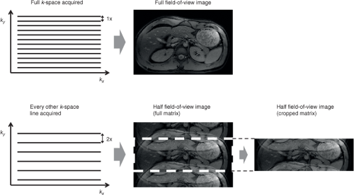
Second, the spacing between k-space points is inversely proportional to the field of view in that direction; the greater the spacing, the smaller the effective field of view (Fig. 5.3). For example, to image faster, a decision is made to skip every other line in k-space. This doubles the spacing between consecutive lines in k-space, and hence half the field of view along the phase encoding direction. The result is an “aliased” image, which means that the image will appear “folded” over itself (Fig. 5.3). Hence, the reconstruction will need to unfold these images or to fill in the missing k-space data to generate a correct image.

Third, k-space is approximately symmetrical across the center. Essentially, if you take one-half of k-space and rotate it 180 degrees around the center, it will look like the other half, except that the phase is opposite. This mirror image between opposite sides of k-space is called Hermitian symmetry.

Fourth, different portions of k-space can be collected separately and pieced together afterward to get an image that looks much better than any of its parts (Fig. 5.2). For example, it is possible to acquire high-spatial-frequency information separately from the contrast-bearing,
low-spatial-frequency information to get the eventual image. This is a powerful tool that allows for great flexibility in inventing new data acquisition schemes. Nonetheless, care must be taken in the design of the MR experiments to ensure that the acquired data are mutually consistent (e.g., the object should be in a similar motion or physiologic state, and the image contents or contrasts should be approximately the same during data acquisition). Otherwise, the inconsistency may lead to artifacts that could manifest as obvious image degradation or, even more problematically, an image that “looks” right but contains incorrect contrast, edge, or physiologic information.

FIGURE 5.2. Different regions of k-space have different effects on the appearance of the image, with the center contributing primarily contrast information, and the periphery contributing more edge information. If the center region of k-space (top left) is used to construct the image (bottom left), the result is a low-resolution image but with excellent contrast information, whereas if only the periphery of k-space (top row, middle) is used, the resultant image has high-resolution edge information but lacks contrast information. Summation of the two yields the full k-space (top right) and correspondingly a full image (bottom right).

How to Use K-Space to Accelerate a Scan or Improve Image Quality

The rest of the chapter describes how modern MRI techniques can significantly improve scan performance by exploiting the properties of k-space outlined previously.

FIGURE 5.3. The spacing between k-space points is inversely proportional to the field of view in that direction; the greater the spacing, the smaller the effective field of view. Here, a full k-space acquisition (top left) yields an unaliased image (top right). Skipping every other line in k-space (bottom left) yields a field of view that is half of the original image. In that case, the object cannot be mapped correctly, and each point in the object is mapped to two locations (bottom middle) in an imaging artifact called aliasing. Displaying the image in the cropped matrix gives the classic “folded over” appearance (bottom right).

Partial Fourier Imaging

Partial Fourier imaging relies on the Hermitian symmetry of k-space, which was exploited very early in the history of MRI to accelerate image acquisition.⁵^,⁶^,⁷ In principle, using this
property, only half of the k-space needs to be collected, as the opposite half can be filled in by copying the symmetric data from the other side of k-space. This kind of “half-Fourier” sampling scheme can be employed in the phase-encoding direction to reduce the number of phase-encoding steps and thus the acquisition time, or in the frequency-encoding direction to shorten the length of data acquisition or echo time and reduce associated artifacts, such as those from T₂^* decay.

In practice, the process of copying information from one part of k-space to the other is imperfect because the symmetry in k-space is not exact owing to phases in the image from magnetic field inhomogeneities, phases in the receiver coils, and patient or physiologic motion. These imperfections degrade the quality of the reconstructed image. To counter this problem, a little more than half of k-space is acquired, so the approach is more correctly called partial Fourier as opposed to half Fourier. The central portion (say, 25%) of k-space is fully sampled on both sides and provides a low-resolution image. The phase of this low-resolution image can be used as an estimate of the phase for the full-resolution image, allowing one to greatly alleviate the phase-related artifacts discussed earlier. If there are phase variations that are not captured by the low-resolution image, artifacts such as signal drops can arise in the reconstructed image. Partial Fourier methods are now ubiquitous in MRI. They are often used “under the hood” in some form to reduce imaging time and/or artifacts and are robust enough that they do not often need to be adjusted from initial, vendor-provided settings for typical clinical exams. Further details of partial Fourier methods are discussed elsewhere.⁸^,⁹

Parallel Imaging

Principle

Parallel imaging¹⁰^,¹¹^,¹² refers to the use of multiple radiofrequency (RF) coils at the same time for signal reception during a scan. It is now included in the standard software on most modern MRI scanners. Parallel imaging is commonly used to accelerate a scan, typically by two- to threefold along each phase-encoding direction at clinical field strengths of 1.5T or 3T.¹³ There are other benefits of parallel imaging, such as reducing geometric distortion in echo-planar imaging¹⁴^,¹⁵ and reducing T₂ blurring in fast spin echoes,¹⁶ among others. These additional benefits, as described later, are linked to how parallel imaging speeds up a scan.

Parallel imaging uses the differences among RF coils to help differentiate signals from different spatial locations. Each RF coil¹⁷ has a localized sensitivity profile, so it only receives signals close to it. Figure 5.4 shows an image of a head, with four coils placed around it. The image acquired with each coil, referred to as the coil image, shows the head shaded by the sensitivity of that coil.

To accelerate a scan, the field of view is set by the scanner to be deliberately smaller than the object along the phase-encoding directions. Reducing the field of view speeds up a scan because it reduces the number of phase-encode lines in the image matrix. For example, to accelerate a scan twofold, the field of view is halved, so the scanner acquires half as many phase-encode lines as the full scan. In effect, it acquires every other line in k-space (Figs. 5.3 and 5.5), so the scan duration is cut in half.

FIGURE 5.4. Example of using four coils (A, B, C and D) around the head for signal reception. Middle row: The image acquired with each coil shows the head shaded by the coil sensitivity. The white arrows point to a set of corresponding locations within the coil images. Note that this location is shaded differently in each coil depending on the sensitivity. The coil sensitivities are different if another set of corresponding locations is examined. Bottom row: Parallel imaging accelerates a scan by reducing the field of view (FOV). In this case, the field of view is halved to accelerate twofold. The reduced field of view leads to aliasing artifacts, which are subsequently removed during reconstruction.

FIGURE 5.5. A closer look at parallel imaging. The left shows the k-space data and corresponding image from one coil. To accelerate the scan twofold, the field of view (FOV) is cut to half. This corresponds to acquiring every-other phase-encode lines of k-space only. The black horizontal lines in k-space in the upper right indicate the skipped lines. With half of the field of view, the image (lower right) shows aliasing artifacts. For a Cartesian acquisition, the aliasing artifacts are simply a superposition of the image with a shifted version of itself. For example, the squares on the lower left image show two locations that are separated by half a field of view. With half the field of view, the two voxel locations are simply superposed in the corrupted image with the aliasing artifacts (lower right). The image-space approach of parallel imaging concerns removing the aliasing artifacts, whereas the k-space approach concerns filling in the missing k-space data. Despite the apparent differences, the two approaches are linearly related.

With the field of view set smaller than the object, the images exhibit aliasing artifacts (Figs. 5.4 and 5.5). Because the coils sense each spatial location differently, the coil sensitivities can be used to differentiate the overlapping signals, which are then assigned to the correct spatial locations to yield an image free of aliasing artifacts. Thus, parallel imaging involves several components:

Multiple RF receiver coils, so that each coil has a different sensitivity over the field of view
Each receiver coil connected to its own receiver chain, so that signals from all coils can be measured in parallel
Fewer phase-encoding steps acquired to speed up a scan, typically by reducing the field of view
Knowledge of the coil sensitivity, so that overlapping signals from different spatial locations can be separated

Image-Space and k-Space Approaches of Parallel Imaging

For historical and conceptual reasons, parallel imaging techniques are generally divided into image-space and k-space approaches. The most commonly used technique in the image-space approach is SENSE (SENSitivity Encoding),¹⁰ and the most common k-space technique is GRAPPA (GeneRalized Autocalibrating Partially Parallel Acquisitions).¹² It should be noted that the two approaches are “linearly related,” just as an image and its k-space data are linearly related. Nevertheless, the two different approaches tackle the reconstruction problem from different angles, which lead to different practical advantages, as described later.

Only gold members can continue reading. Log In or Register to continue