MR Relaxation Theory and Exchange Processes in the Presence of Contrast Agents
Joel R. Garbow
Joseph J.H. Ackerman
Introduction
As outlined throughout other chapters in this book, the focus of most clinical nuclear magnetic resonance (NMR or, more commonly, MR) procedures is on the imaging of water found within tissue. Thus, when one refers to MR imaging of the brain, one really means hydrogen (1H, proton) MR imaging of the water in the brain. Water is ubiquitous (∼75%) in biological tissue; its high concentration (∼0.75 × 110 molar [M] equivalent 1H) makes it an attractive target for MR imaging. The challenge becomes one of generating sufficient contrast to allow visualization of detailed structures and substructures within tissue. Fortunately, the MR properties of water are exquisitely sensitive to the local environment, a sensitivity that is exploited to generate image contrast. This chapter describes the use of exogenous relaxation agents to enhance MR image contrast (“contrast agents”). It begins with a review of MR relaxation, characterized by exponential time constants T1, T2, and T2*, and describes how differences in relaxation among water 1H spins in different local environments can serve as important sources of contrast. The chapter then reviews the requirements for effective relaxation and describes MR relaxation in multicompartment, exchanging systems. Next, magnetization transfer (MT), a process that can drive contrast in biological systems, including chemical exchange saturation transfer (CEST) and CEST using paramagnetic agents (PARACEST), is introduced. This sets the stage for a description of molecular relaxation agents, including a discussion of their magnetic properties, how their efficacy is assessed, and considerations of agent biodistribution and safety. The chapter then discusses nanoscale materials as contrast agents, including the efficacy, biodistribution, and safety of superparamagnetic iron oxides, and concludes with a brief discussion of relaxation agents in perfusion imaging.
MR Relaxation: An Empirical View
General Considerations
Relaxation is the return to equilibrium from any nonequilibrium (perturbed) state. Many relaxation phenomena, including those related to temperature, concentration, pressure, and mechanical stress/strain, are familiar in everyday life. Here, relaxation is discussed specifically as it applies to a collection of nuclear spins (nuclear magnetic dipoles) within a strong static magnetic field, B0. Initially, relaxation is discussed in terms of MR spectroscopy, though precisely the same considerations apply to imaging experiments. The first question is, “What do we know about the magnetization of water, M(t) (or, more precisely, the population of hydrogen [1H] nuclear spins of water) at thermal equilibrium?” Consider the following Gedanken experiment: Place a tube of water into B0 of an MR scanner and go out for a cup of coffee (formally, a “long enough” period, t =∞, which for 1H MR is a few seconds), returning once the sample is at thermal equilibrium. Among the questions one might ask are (a) “In what direction does the vector describing the net water 1H magnetic moment point?” and (b) “What signal, if any, is sensed by the receiver coil that serves as the signal detector?” The answers to these questions are (a) “The water 1H magnetic moment is stored (aligned, polarized) along the B0 axis (by convention, the longitudinal or z-axis), to an extent defined by the Curie law, Mz(∞) = Mz(Curie)” and (b) “There is no observable signal because there is no coherent component of the water magnetic moment in the transverse plane, Mxy(∞) = 0.” Note that the transverse (x-y) plane lies perpendicular to the direction (z-axis) of B0 and that MR receiver coils only detect a magnetic moment’s transverse component, Mxy(t), which precesses at the Larmor (resonance) frequency about B0. This condition, with the net Curie law magnetization pointed along B0, characterizes a spin system at equilibrium.
Transverse Relaxation
The basic MR experiment (imaging or spectroscopy) begins with the application of one or more radiofrequency (RF) pulses to perturb the spin population from its equilibrium alignment along B0. In the simplest case, the effect of the RF pulses is to nutate the net magnetic moment so that it is positioned in the x-y plane, perpendicular to B0. This transverse magnetic moment will immediately precess about B0, thus oscillating within the x-y plane at its characteristic (resonance or Larmor) frequency, generating a voltage (measurable signal) in the receiver coil, as illustrated in Figure 6.1A. With time, the observable signal dies away as the x-y coherence of the magnetic moment, Mxy(t), decays to zero, its equilibrium value. The envelope of this decay is shown in Figure 6.1B. In many chemical and biological systems, the approach to equilibrium can be described as a mono-exponential decay, Eq. [1],
characterized by the transverse relaxation rate constant, R2*, or its inverse, the transverse relaxation time constant T2* (=1/R2*):
characterized by the transverse relaxation rate constant, R2*, or its inverse, the transverse relaxation time constant T2* (=1/R2*):
where Mxy(0) is the initial transverse component of the magnetic moment at time zero (i.e., immediately following the perturbing RF pulse[s]).
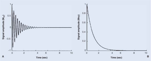 FIGURE 6.1. A: Signal amplitude (Mxy) vs. time (free induction decay, FID) for an ensemble of nuclear spins following excitation with a 90-degree radiofrequency (RF) pulse. B: Envelope of the signal amplitude for the FID shown in A. For many spin systems, the decay of signal is described by a mono-exponential function, characterized by the decay rate constant R2 or R2* and its inverse, the transverse relaxation time constant, T2 or T2*. |
The decay of the magnetic moment’s transverse coherence is composed of two different components: (a) irreversible decay, the component that cannot be refocused/recovered with a 180-degree (π) pulse/echo and which is principally due to random, molecular motion–modulated, spin–spin interactions, and (b) reversible decay, the component that can be refocused with a π pulse/echo and which is principally due to static inhomogeneities (gradients) in the local magnet field arising from mesoscopic magnetic susceptibility inhomogeneities (e.g., parenchyma vs. vascular bed containing oxygenated blood or contrast agent) or macroscopic global inhomogeneities in B0 (e.g., magnet shimming). In terms of nomenclature, the total transverse magnetization decay-rate constant is designated as R2* (“R two star”), the rate constant describing irreversible decay is R2, and the rate constant describing reversible decay is R2′ (“R two prime”). Because rate constants are additive (time constants are not), one can write:
In general, gradient-echo experiments are sensitive to R2*, whereas spin-echo experiments are sensitive to R2.
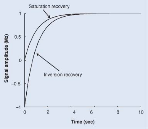 FIGURE 6.2. Recovery of z-magnetization (Mz) as a function of time for an ensemble of nuclear spins following either inversion or saturation of the magnetization. For many spin systems, the recovery of signal is described by a mono-exponential function, characterized by the rate constant R1 and its inverse, the longitudinal relaxation time constant, T1. |
Longitudinal Relaxation
As noted previously, the equilibrium condition for a collection of nuclear spins is a net alignment or polarization along the direction of B0, that is, Mz(∞)=Mz(Curie). Like transverse relaxation, the return of a perturbed/nonequilibrium state of Mz(t) to its thermal equilibrium value is frequently characterized by a mono-exponential time dependence, illustrated schematically in Figure 6.2. The longitudinal relaxation rate constant characterizing this process is R1; its inverse is the longitudinal relaxation time
constant, T1 = (1/R1), and Eq. [3] describes longitudinal relaxation:
constant, T1 = (1/R1), and Eq. [3] describes longitudinal relaxation:
where, as before, Mz(∞) is the equilibrium value (Curie law) of the z-axis magnetic moment, and Mz(0) is the initial value of the z-axis magnetic moment immediately following the perturbation from equilibrium. As suggested by Figure 6.2, T1 measurements often begin with either an inversion of the net magnetic moment so that it is aligned antiparallel with respect to B0 (“inversion recovery”) or with a saturation of the net magnetic moment so that the initial value is zero (“saturation recovery”), although there are many other measurement protocols in use. The relaxation rate constant describing the recovery of the magnetization is independent of the initial nonequilibrium state of z-magnetization.
Relaxation as a Source of Contrast
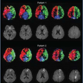
Differences in either T1 or T2 relaxation time constants can serve as important sources of image contrast. Consider the image of a sample containing two tissues, A and B, present in equal amounts, and having the same density of water. In a proton density (1H density) image, collected with a very long repetition time (TR) between scans (i.e., between RF pulses that perturb spin-state populations), the image intensities of signal arising from tissues A and B will be equal (yielding zero contrast). However, as illustrated in Figure 6.3A, if tissues A (black curve) and B (red curve) have different T1 relaxation time constants, significant contrast (image intensity differential) can be generated by an appropriate choice of TR. In Figure 6.3B, contrast, defined as (SignalA – SignalB), is plotted in blue, as a function of TR. The value of TR corresponding to maximum contrast is indicated by a black arrow. Differences in T2 (or T2*) can be exploited, in a similar manner, to generate image contrast in experiments by varying the time to echo (TE). Considering the water 1H MR signal from mammalian tissues and fluids, tissues and fluids with long T1 generally also have long T2, and vice versa. Recalling that long T1 generally results in diminished signal intensity, and long T2 generally results in enhanced signal intensity, it follows that T1-weighted and T2-weighted images of the same body location can have very different, even inverted, contrasts. A classic example is shown in Figure 6.3, where T1-weighted (panel C) and T2-weighted (panel D) images show completely opposite contrasts for the same slice of a human brain.
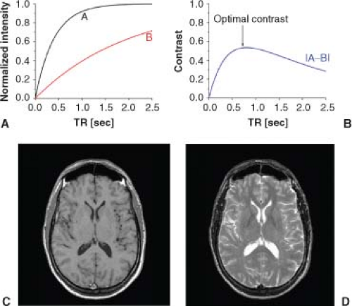 FIGURE 6.3. A: Recovery of z-magnetization (Mz) as a function of pulse sequence repetition time (TR) for two different ensembles of spins, “A” and “B,” having longitudinal relaxation time constants (T1) of 400 ms and 2000 ms, respectively. B: Contrast, |(Signal intensity)A − (Signal intensity)B|, as a function of TR, assuming equal numbers of A and B spins. The optimal contrast, at TR = 800 ms, is indicated by the black arrow. Bottom: Single slices from (C) T1-weighted and (D) T2-weighted images of human brain. The same anatomic slice is displayed in both of these images; the differences in their appearance arise from the differences in T1 and T2 relaxation time constants for white matter, gray matter, and cerebral spinal fluid. (Images courtesy of Dr. Jeffrey J. Neil, Washington University School of Medicine, Saint Louis, MO.) |
MR Relaxation: The Physical Underpinnings
General Considerations
Now that a brief overview of longitudinal and transverse relaxation and of how the relaxation time constants T1 and T2 are defined and measured has been provided, the chapter may turn to a discussion of the requirements for effective (i.e., rapid) relaxation. An understanding of the factors that are important for efficient nuclear-spin relaxation will lay the groundwork for understanding the role of relaxation/contrast agents and the characteristics required of effective contrast agents. As before, in this discussion, the focus is on the relaxation of hydrogen spins in water molecules within biological tissue.
Transverse Relaxation
The net 1H magnetic moment for an ensemble of water molecules is the vector sum of the nuclear-spin magnetic dipoles from water in all of its local environments. Immediately following an RF pulse, all of the individual spin vectors point in the same direction—that is, they are “in phase” in the transverse plane. As a result of differences in the local magnetic fields experienced by the spins (variations over angstrom, nanometer, or micrometer length scales), which generate different precession frequencies within an imaging voxel, these spin vectors dephase and the net transverse coherence (vector sum) of the magnetic moment shrinks. As noted earlier, this signal decay—due to loss of phase coherence—can arise from either irreversible (spin–spin; R2) processes or reversible (static; R2′) processes. Spin–spin magnetic interactions—inherent to T2 decay—can be thought of as producing
stochastic (random), fluctuating (modulated by molecular motions), microscopic-scale field inhomogeneities, occurring over distances characteristic of atomic/molecular lengths (i.e., angstroms). These fluctuating magnetic fields can be described in terms of a “correlation time” (also referred to as the memory time), τc, which describes how long, on average, a given spin–spin magnetic interaction exists at a particular energy (strength of interaction). A short τc implies short memory or high-frequency modulation, while long τc implies long memory or low-frequency modulation. Variations in the local magnet field can also arise from macroscopic-scale inhomogeneities, those occurring over distances larger than an imaging voxel. Examples would be static B0 inhomogeneities caused by imperfect shimming of B0 or large-scale magnetic susceptibility variations, such as those at air–tissue interfaces. Mesoscopic-scale inhomogeneities are those occurring over distances smaller than an imaging voxel but much larger than molecular scales. An example would be inhomogeneities owing to blood vessel networks in brain tissue. Macroscopic-scale inhomogeneities are generally undesirable, because they can degrade image quality and provide no information of biologic interest, while mesoscopic-scale inhomogeneities are responsible for blood level oxygen dependence (BOLD) contrast1 that drives all of functional MR imaging (MRI).2,3
stochastic (random), fluctuating (modulated by molecular motions), microscopic-scale field inhomogeneities, occurring over distances characteristic of atomic/molecular lengths (i.e., angstroms). These fluctuating magnetic fields can be described in terms of a “correlation time” (also referred to as the memory time), τc, which describes how long, on average, a given spin–spin magnetic interaction exists at a particular energy (strength of interaction). A short τc implies short memory or high-frequency modulation, while long τc implies long memory or low-frequency modulation. Variations in the local magnet field can also arise from macroscopic-scale inhomogeneities, those occurring over distances larger than an imaging voxel. Examples would be static B0 inhomogeneities caused by imperfect shimming of B0 or large-scale magnetic susceptibility variations, such as those at air–tissue interfaces. Mesoscopic-scale inhomogeneities are those occurring over distances smaller than an imaging voxel but much larger than molecular scales. An example would be inhomogeneities owing to blood vessel networks in brain tissue. Macroscopic-scale inhomogeneities are generally undesirable, because they can degrade image quality and provide no information of biologic interest, while mesoscopic-scale inhomogeneities are responsible for blood level oxygen dependence (BOLD) contrast1 that drives all of functional MR imaging (MRI).2,3
T2′ relaxation can also arise from the presence of paramagnetic materials, such as iron oxides or lanthanides (Gd), suggesting these materials as potential T2* contrast agents. The dephasing effect of tissue-induced perturbations in magnetic field homogeneity is typically linear in field strength (i.e., greater at higher field). The magnetic field perturbations arising from iron oxide particles extend over distance scales very large compared to molecular dimensions. Thus, paramagnetic iron oxide T2* contrast agents have a significantly longer-range effect than molecular complexes of Gd(III)-based T1 contrast agents (vide infra). As discussed in greater detail later, gadolinium chelates and superparamagnetic iron oxide nanoparticles injected intravenously can be used to measure tissue perfusion and act as “negative” contrast agents, producing hypointensity (loss of signal in T2*-weighted images) in tissues in which they accumulate. Cells (e.g., mesenchymal stem cells, T cells) labeled with iron oxide particles can also be tracked by T2*-sensitive methods.
Longitudinal Relaxation
There are two factors of primary importance in longitudinal (T1) MR water relaxation: (a) the water 1H nuclear magnetic dipoles must experience magnetic interactions with the surrounding molecular environment (i.e., there must be a magnetic coupling of the 1H nuclear magnetic dipoles of water to the surrounding “lattice”), and (b) the local magnetic interactions must fluctuate with time (i.e., the interactions must be time modulated). If either of these conditions (magnetic interaction/coupling to the lattice or fluctuations thereof) is poorly met, relaxation will be inefficient (slow). For longitudinal relaxation, characterized by the rate constant R1, one can write:
where E is the average strength (energy) of the local magnetic lattice interactions experienced by the spins of interest and fn(τc) is a function that describes the modulation of E in time, expressed in terms of the correlation time, τc, described previously. Note that R1, being proportional to (E)2, depends strongly on the strength of the local magnetic interactions.
For water 1H MR relaxation, the dominant magnetic interaction is the through-space dipolar interaction, in which the population of water 1H magnetic dipoles senses the magnetic fields arising from nearby nuclear or electron magnetic dipoles on other molecules (i.e., the surrounding lattice). As illustrated schematically in Figure 6.4A, the energy of interaction, Edd, is proportional to the size of the interacting dipoles and to the inverse of the cube of the distance (r) between dipoles—that is, Edd is proportional to r−3, leading to an r−6 dependence for R1. Edd is also proportional to [1 − 3 cos2(θ)], where θ is the angle of the vector connecting the two dipoles relative to the B0, though the rapid, isotropic tumbling of water molecules in solution averages this angular dependence.
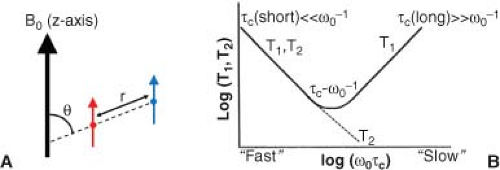 FIGURE 6.4. Left: The direct, through-space coupling between a pair of magnetic dipoles is proportional to the size of the interacting dipoles, to the inverse cube of the distance (r) between them, and to [1 − 3 cos2(θ)], where θ is the angle of the vector connecting the two dipoles relative to the B0. Rapid, isotropic tumbling of water molecules in solution averages this angular dependence. Right: The dependence of the relaxation time constants T1 and T2 on the correlation (memory) time, τc, as described by the equations in Geek Box 6.1, plotted as log(relaxation time constant) versus log of the unitless quantity ω0τc, where ω0 = 2πν0 (ν0 = 1H Larmor frequency). The minimum value for T1 occurs when τc = ω0−1. For faster motions (τc < ω0−1), both T1 and T2 increase, whereas for slower motions (τc > ω0−1), T2 continues to decrease, and T1 again increases. |
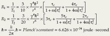
As described previously, the modulation of the interaction required to cause relaxation is expressed in terms of a motional correlation or memory time, τc. A derivation of the dependence of the longitudinal and transverse relaxation time constants on correlation time based on the Bloembergen-Purcell-Pound (BPP) relaxation theory, detailed elsewhere,4,5,6,7,8 is beyond the scope of this article. The Geek Box summarizes the functional form of this dependence for both R1 and R2 resulting from intramolecular dipole–dipole interactions. The important qualitative observation is that the expression for R1 relaxation contains magnetic field strength–dependent terms,
whereas R2 contains both field strength–dependent terms and a zero-frequency term. Recalling that ω0 = γB0 defines the Larmor (resonance) frequency, R1 has maxima (corresponding minima in T1) for the conditions τc = ω0−1 and τc = (2ω0)−1. For longer or shorter τc, relaxation is less efficient. The dependence of T1 and T2 on ω0τc is plotted schematically in Figure 6.4B. Note, in the special case of intramolecular dipole–dipole-induced relaxation when τc is very short (ω0τc≪1), a condition referred to as “extreme narrowing,” the relaxation rate constants R1 and R2 are equal and are directly proportional to τc; that is, they are independent of ω0.
whereas R2 contains both field strength–dependent terms and a zero-frequency term. Recalling that ω0 = γB0 defines the Larmor (resonance) frequency, R1 has maxima (corresponding minima in T1) for the conditions τc = ω0−1 and τc = (2ω0)−1. For longer or shorter τc, relaxation is less efficient. The dependence of T1 and T2 on ω0τc is plotted schematically in Figure 6.4B. Note, in the special case of intramolecular dipole–dipole-induced relaxation when τc is very short (ω0τc≪1), a condition referred to as “extreme narrowing,” the relaxation rate constants R1 and R2 are equal and are directly proportional to τc; that is, they are independent of ω0.
Geek Box: Longitudinal and Transverse Relaxation Rate Constants
At typical clinical MRI field strengths, semisolids (e.g., tissue) display strong field strength–dependent T1 relaxation time constants (longer T1 at higher field), while the T1 values of fluids (e.g., cerebrospinal fluid [CSF]) and solids (e.g., bone) are only weakly field strength dependent.
In Vivo Measurement of R1 and R2 Relaxation
The accurate measurement of R1 and R2 relaxation in solution and in phantoms, including plasma, can provide important characterization of paramagnetic contrast agents and their properties. Before discussing the characteristics of paramagnetic agents in greater detail, the chapter describes briefly various challenges associated with measuring R1 and R2 relaxation in vivo and some of the strategies developed for meeting these challenges.
Accurate measurement/mapping of longitudinal (R1) relaxation can provide important tissue characterization, is useful for choosing optimal imaging parameters, and is needed to quantitatively analyze experiments such as dynamic contrast–enhanced MRI. Various different methods exist for measuring longitudinal relaxation in vivo.9,10 As described previously, T1 is often measured by inversion recovery (IR) or saturation recovery (SR) techniques, via a series of experiments measuring the return of magnetization to equilibrium following an excitation RF pulse. Inversion recovery and saturation recovery methods are readily incorporated into spin-echo imaging sequences. Although highly accurate, the resulting experiments for measuring T1 are often too time-consuming to be applied in vivo. Fast inversion recovery11 and Look-Locker methods12,13,14,15 are variants on these basic IR experiments, designed to reduce the time required to perform these measurements while preserving accuracy. Variable flip-angle experiments are a second class of methods for measuring T1,16,17 in which signal is measured as a function of the flip angle of the initial excitation pulse and fitted to an appropriate signal equation. Although much faster than IR experiments, variable flip angle measures are more susceptible to errors, especially those owing to spatial inhomogeneity of the RF excitation pulses.
MR Relaxation in Multicompartment Exchanging Systems
MR in Complex Systems
Mammalian tissue is a complex microarchitecture composed of various components, including cells, structural matrix, and vasculature. It follows that the 1H tissue-water MR signal from mammalian tissue is the sum of water signals originating from multiple compartments—intracellular, extracellular, vascular, matrix associated—with different MR properties. Here, the simple but illustrative case in which the MR signal is the sum of signals from two well-mixed (uniformly distributed) compartments, each with different relaxation properties but the same resonance frequency, is briefly considered.
First, the reader is reminded that compartments, which are here defined as identifiable, distinct, spin systems, can communicate in two ways: (a) via physical or chemical exchange of 1H magnetization, as when a water molecule initially in compartment A moves into compartment B (and vice versa), and (b) via through-space exchange of magnetization, as when water 1H magnetization in compartment A senses the state of the 1H magnetization in compartment B via the dipole–dipole interaction. The characteristics of the observed MR signal depend critically on the rate constants governing the communication between compartments (i.e., the rate constants governing magnetization exchange).
Nonexchanging Compartments
If the two compartments are not exchanging magnetization, then the signal describing the relaxation characteristic(s) of the two-spin systems is found to be simply the sum of relaxation-monitoring signals arising from the two compartments. For example, consider that compartment A is characterized by large R2* (rapid, mono-exponential decay of transverse magnetization, i.e., rapid signal decay) and compartment B by small R2* (slow, mono-exponential decay of transverse magnetization, i.e., slow
signal decay). Consider further that 50% of the water resides in each of the two compartments. The relaxation-monitoring signal from this nonexchanging, two-compartment system will exhibit a biexponential decay, with the amplitude of the rapidly (mono-exponentially) decaying component equal to the amplitude of the slowly (mono-exponentially) decaying component (i.e., 50%:50%). Figure 6.5 shows the observed decay of signal for compartments A and B under the assumption of nonexchanging compartments (blue curve) and fast exchange (red curve). The inset on this figure shows these same data on a semilogarithmic plot.
signal decay). Consider further that 50% of the water resides in each of the two compartments. The relaxation-monitoring signal from this nonexchanging, two-compartment system will exhibit a biexponential decay, with the amplitude of the rapidly (mono-exponentially) decaying component equal to the amplitude of the slowly (mono-exponentially) decaying component (i.e., 50%:50%). Figure 6.5 shows the observed decay of signal for compartments A and B under the assumption of nonexchanging compartments (blue curve) and fast exchange (red curve). The inset on this figure shows these same data on a semilogarithmic plot.
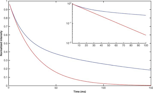 FIGURE 6.5. Relaxation curves (signal intensity vs. echo time, TE) for a spin system consisting of two species, A and B, present in a ratio of 1:1 with equivalent resonance frequencies and having T2 values of 15 ms (T2A) and 150 ms (T2B), respectively. For the case of no exchange between species, biexponential signal decay, with decay rate time constants T2A and T2B, is observed (blue curve). In the case of fast exchange between species, a mono-exponential decay is observed, with a decay rate constant equal to the algebraic average of T2A and T2B (red curve). The inset shows an expanded view of these same data on a semilog plot. |
Slow Exchange
When compartments with different MR properties begin to exchange magnetization, they start to lose their distinct MR identities. In the case of two compartments, compartment A acquires some of the MR characteristics of compartment B and vice versa. Considering the case discussed previously, when exchange is slow, the observed transverse magnetization (the signal) is still characterized by biexponential decay; however, the individual component mono-exponential signal decay rate constants and amplitudes are not those that would be measured if the compartments were nonexchanging. Rather, the large rate constant will be a bit smaller, the small rate constant a bit larger, the large amplitude a bit smaller, and the small amplitude a bit larger. In short, the MR characteristics of the two compartments will begin to merge. Slow exchange, in which relaxation is much faster than magnetization exchange between compartments, is generally defined by the condition in which the sum of the rate constants governing exchange between the two compartments (kA + kB) is much less than the sum of the relaxation rate constants for the two compartments in the absence of exchange (R2A* + R2B*): In this example, (kA + kB) ≪ (R2A* + R2B*). Note that by manipulating the sum (R2A* + R2B*), for example, by adding contrast agent in one compartment, one can change the MR exchange condition without changing the actual kinetic exchange rate constants, a feature that is often overlooked.
Fast Exchange
In the fast exchange condition, in which magnetization exchange between compartments is much faster than relaxation, the MR experiment only senses the mole fraction (population fraction)–weighted dynamic average of the relevant MR property for each compartment. For example, consider the observed signal decay for the two-compartment case when (kA + kB) >> (R2A* + R2B*). Here, the relaxation-monitoring signal profile is characterized by a mono-exponential decay with rate constant R2* given
by the mole fraction–weighted average of R2A* and R2B*; that is,
by the mole fraction–weighted average of R2A* and R2B*; that is,
where Xa and Xb are the mole fractions (population fractions) of water in compartments A and B, and R2A* and R2B* are again the relaxation rate constants for the two compartments in the absence of exchange.
Many complex, multicompartment systems are well fit by biexponential relaxation (R1, R2, or R2*) profiles. It is tempting, although often incorrect, to assume that one is dealing with a simple, two-compartment system that is either not exchanging or is in slow exchange. Caveat emptor!
Intermediate Exchange
Expressions governing multicompartment spin systems in intermediate exchange are more complicated and are not dealt with here. Suffice it to say that averaging of the relaxation properties of the compartments involved is incomplete and the relaxation signal profiles require more sophisticated analysis to extract the MR relaxation and exchange parameters of interest. A further complication arises when the populations of exchanging water 1H spins in the two (or more) compartments have different, compartment-specific resonance frequencies. Such considerations are beyond the scope of this chapter but are covered in many standard texts.8,18
MR Magnetization Transfer and Chemical Exchange Saturation Transfer
Magnetization Transfer
As described earlier, most clinical MRI experiments focus on the imaging of 1H spin populations in mobile tissue water characterized by relatively long T2* values. A long T2* implies slow decay of transverse magnetization and would yield a narrow resonance lineshape in an MR spectroscopy experiment. However, biological samples and tissues also contain membranes and macromolecules (e.g., proteins) that contain many 1H spins. These immobile spin populations are generally not observed directly in MRI experiments designed to detect mobile spins owing to incomplete molecular motion–driven averaging of the coupling (magnetic interactions) among the immobile 1H spins, which leads to very short T2* values. A short T2* implies a fast decay of transverse magnetization and would yield a broad resonance lineshape in an MR spectroscopy experiment. Nonetheless, the macromolecule 1H magnetization can interact with, and thus can affect the relaxation of, tissue-water 1H magnetization and, thereby, serve as a significant source of contrast in imaging experiments, through a process known as magnetization transfer.9,19
Although there are many variations on the theme, consider an experiment in which the very broad 1H resonance lineshape associated with tissue macromolecules (the macromolecular matrix) is irradiated far (∼5 kHz) off-resonance relative to the mobile water signal with a continuous weak RF pulse (or a train of short, off-resonance pulses). As a result of strong 1H–1H dipolar coupling within the immobile spin population, this RF irradiation will lead to a saturation of the 1H spins within the entire macromolecular matrix while having a small, though nonnegligible, direct effect on the mobile water signal (because the irradiation is far off-resonance for the 1H spins of water). However, of more import, if the macromolecular spins communicate with the mobile water 1H spins, either by dipolar relaxation (cross-relaxation)—energy-conserving spin flips (spin A “up”/spin B “down” → spin A “down”/spin B “up”) between neighboring 1H spins—or direct chemical exchange, the saturation of the macromolecular spin population polarization (Mz = 0) can be transferred to the water, leading to a loss of observable water signal intensity. The difference in observed water signal intensity for experiments conducted with and without the off-resonance RF saturation pulse (or with a control-state RF pulse whose frequency is chosen to not excite/saturate spins in the macromolecular matrix) provides a measure of magnetization transfer between spins of the macromolecular matrix and water. This difference in signal intensities can be modeled in terms of the magnetization transfer rate constant governing exchange between the macromolecular matrix and water, and the R1 relaxation rate constants in the absence of MT for the 1H spins of the immobile macromolecular matrix and the mobile-water pool. Modeling of MT data must also take into account the direct effects of off-resonance irradiation on the 1H spins of mobile water.
MT can serve as an important source of image contrast and has been used to characterize various different disease states.20,21,22,23,24,25,26,27 As described later, CEST28,29,30,31 and PARACEST32,33,34 are based on the basic principles of magnetization transfer. MT effects can also complicate the quantitative interpretation of other experiments that involve the use of saturation pulses. For example, arterial spin labeling (ASL),35,36,37,38,39 a method for measuring blood flow and tissue perfusion that is the subject of Chapters 15 through 22 in this volume, involves using continuous or pulsed RF irradiation to saturate the 1H spins in blood (water) in a well-defined excitation plane. However, this same RF radiation will also saturate spins in macromolecules within and out of the excitation plane. MT effects, as described previously, can shorten the apparent T1 of blood, thereby changing the apparent perfusion parameters derived from ASL experiments. As a consequence, these experiments must include well-balanced control experiments so that the ASL-derived perfusion parameters are accurate, and not confounded by MT effects.
Chemical Exchange Saturation Transfer
As described later, contrast agents that are built around paramagnetic centers, including Gd and Fe, are always “on,” in the sense that the relaxation/dephasing effects of the unpaired electrons are continually experienced by all 1H spins in water molecules that are proximate to the agents. However, magnetization transfer from saturated spins to the 1H of mobile water produces contrast effects that are driven by RF irradiation, suggesting MT as the basis for generating switchable (on/off) contrast agents. Clearly, the ability to switch a relaxation effect on and off is a powerful feature that can add significantly to an agent’s versatility. The development and use of CEST and PARACEST agents, which function via an MT mechanism and can be turned on and off via switchable RF irradiation, is a growing, active area of MRI research. Although the details of these CEST and PARACEST methods are beyond the scope of this chapter, a very brief introduction to these techniques is provided here.
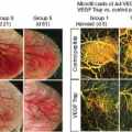
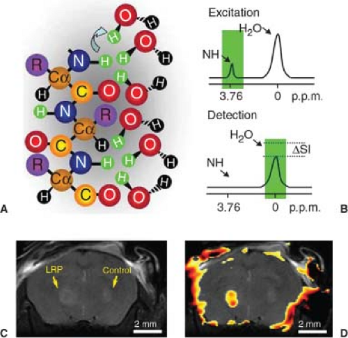 FIGURE 6.6. Lysine-rich protein (LRP) as a chemical exchange saturation transfer (CEST) reporter. A: Schematic representation of a hydrated LRP. B: Frequency-selective radiofrequency (RF) pulses label (green) the amide 1H. These 1H spins exchange with water 1H spins, thereby reducing magnetic resonance imaging (MRI) signal intensity (ΔSI). LRP-expressing and control xenografts were injected in opposite hemispheres of severe combined immunodeficiency (SCID) mouse brains. C: Anatomic image of resulting mouse brain. D: CEST signal intensity difference map overlaid on the anatomic image distinguishes LRP-expressing and control xenografts. (Reproduced, with permission, from Gilad AA, McMahon MT, Walczak P, et al. Artificial reporter gene providing MRI contrast based on proton exchange. Nat Biotechnol. 2007;25[2]:217–219.) |
A CEST agent is a molecule (either exogenous or endogenous) having one or more exchangeable 1H (exchangeable with a water 1H) whose 1H resonance is at a frequency significantly different from that of bulk water. The magnetization from these exchangeable protons can be saturated by RF irradiation, and the saturation can be transferred via chemical exchange to nearby mobile water molecules, leading to a diminution in its signal. Thus, the effects of CEST contrast agents can be switched on and off via RF irradiation (i.e., the signal intensity of the mobile water protons is reduced only when the exchangeable protons of the CEST agent are irradiated/saturated), under direct experimental control. Figure 6.6 illustrates the use of CEST imaging to detect, in vivo, a reporter gene that encodes a lysine-rich protein (LRP) reporter in mouse brain.
Two limitations of CEST and CEST agents are that (a) the difference in resonance frequency between the exchangeable 1H spins of the CEST agent and the 1H spins of mobile water, Δω, is often small, leading to direct, unwanted saturation of the water signal; and (b) the requirement that Δω > kex, where kex is the rate constant governing exchange between 1H spins of the CEST agent and the 1H spins of mobile water, can be difficult to achieve, especially at low field. Both of these limitations can be overcome by increasing the chemical shift range (Δω) of the exchangeable 1H spins of the CEST agent by building CEST agents around paramagnetic, lanthanide metal centers that serve as chemical (frequency) shift agents. Examples of such lanthanides include Pr3+, Nd3+, Sm3+, Eu3+, Tm3+, and Yb3+; the chemical shifts of chelated, 1H-containing complexes built around these lanthanides span a chemical shift range of greater than 500 ppm. Because they contain a paramagnetic ion, the resulting, RF-switchable contrast agents are referred to as PARACEST agents.
Molecular Contrast (Relaxation) Agents
Magnetic Properties
Contrast agents are generally classified as either paramagnetic or superparamagnetic. The response of a material to an applied magnetic field, its induced bulk magnetic moment, is defined by its magnetic susceptibility χ (see Geek Box). The magnetic susceptibility of diamagnetic materials (no unpaired electrons) is small and negative (χ ≈ −10−6 − 10−9; the negative sign implies that diamagnetic material opposes/reduces B0). Most tissue, biological fluids, and proteins are diamagnetic and the relaxation times of the 1H spins of water in these materials are long (e.g., T1 and T2 relaxation time constants of pure, degassed water are approximately 4 seconds).
Atoms that have unpaired electrons in their outer electron orbitals have a nonzero electron magnetic moment. When placed in an external magnetic field, these materials acquire a net magnetization in a similar fashion to that observed for the 1H nuclear spin.
For example, gadolinium (Gd3+) has seven unpaired electrons in its 4f orbital and iron (Fe3+) has five unpaired electrons in its 3d orbital. Paramagnetism is generally defined by two magnetic properties. First, paramagnetic
materials have a positive magnetic susceptibility (adds to the applied field) that is directly proportional to the external field, meaning that the induced magnetization increases linearly with increasing external magnetic field. Second, in the absence of an external magnetic field, the individual magnetic moments are randomly oriented, producing no net magnetization. Paramagnetic metal ions can serve as both T2 (enhance decay of transverse magnetization; loss of signal) and T1 (shorten T1; increase of signal) agents.
materials have a positive magnetic susceptibility (adds to the applied field) that is directly proportional to the external field, meaning that the induced magnetization increases linearly with increasing external magnetic field. Second, in the absence of an external magnetic field, the individual magnetic moments are randomly oriented, producing no net magnetization. Paramagnetic metal ions can serve as both T2 (enhance decay of transverse magnetization; loss of signal) and T1 (shorten T1; increase of signal) agents.
Geek Box: Magnetic Susceptibility
For a homogeneous, isotropic material (e.g., liquid water),
where χ is the magnetic susceptibility of the material, B0 is the applied magnetic field, and M is the net magnetization of the material at clinical temperatures.
Diamagnetic materials: χ is slightly negative (<0); M scales linearly with B0; at zero applied magnetic field strength, M is 0.
Paramagnetic materials: χ is positive (>0); M scales linearly with B0; at zero applied magnetic field strength, M is 0.
Superparamagnetic materials: M reaches a saturation magnetization (Msat) at clinical scanner field strengths where χ >>0, approximately 10 times greater than for paramagnetic materials; at zero applied magnetic field strength, M is 0.
Ferromagnetic materials: M reaches a saturation magnetization (Msat) at clinical fields, where χ>> 0; at zero applied magnetic field, M is >0.
As noted previously, contrast agents may be used to modulate the longitudinal and transverse relaxation rates of water 1H in various tissues. Table 6.1 lists the names and properties, including structure, ionicity, and relaxivity, of contrast agents that are clinically available or are in clinical testing.
Related posts:
Stay updated, free articles. Join our Telegram channel

Full access? Get Clinical Tree


