MR Spectroscopy and the Biochemical Basis of Neurologic Disease
Eva-Maria Ratai
R. Gilberto González
Introduction
The purpose of this chapter is to provide practical guidance in the clinical application of proton MR spectroscopy (MRS) of the brain. It must be understood at this point in the maturation of clinical MR that MRS is only an adjunctive tool in the diagnostic neuroradiology armamentarium. Despite the initial excitement about the specificity and added value of metabolic information, the reality is that MRS has value, but that value is complementary and only rarely trumps other imaging findings. The radiologist employing this tool in the clinical setting must certainly keep foremost in mind that the information provided by MRS is properly interpreted only when all of the imaging and clinical information is incorporated.
Key Concept: Always interpret the MR spectrum in light of other imaging data.
This chapter is designed to be self-contained although some topics are covered in more detail elsewhere in this book. The focus is on 1H MRS because it is the method that is widely available clinically. The chapter covers the physics of MRS, the chemistry of the MR spectrum, technical aspects of in vivo brain MRS, and the biologic basis of the normal and abnormal brain spectrum. The chapter concludes with current clinical applications which we have divided into three classes based on practical considerations. This classification arises from the major limiting factor in using this technique: the low signal-to-noise ratio (SNR) of the brain proton MR spectrum. The concentrations of the metabolites measured by 1H MRS are some 10,000 times lower in concentration than water, and explains the three to four orders magnitude difference in SNR between MRS and MRI. The low SNR results in low spatial resolution and significant error in the measurement of peak heights or areas.
Key Concept: The low SNR of in vivo MRS results in low spatial resolution and significant error in the measurement of peak heights or areas.
The clinical applications of MRS are divided into three classes: Class A MRS applications are those circumstances in which the interpretation of the MR spectrum is of value in individual patients. Because of the SNR, an abnormal MR spectrum is usually only obvious in the case of a qualitative or large quantitative change. An example of the former would be the presence of a prominent lactate resonance in the case inborn errors of metabolism, and an example of the latter would be the high increase in the choline resonance in a high-grade glioma. Indeed, it is in the evaluation of brain masses and inborn errors of metabolism that MRS is most useful in individual patients and is the major subset of Class A applications. There are neurologic diseases where the changes in the MRS spectrum are occasionally large enough that they may be useful for clinical management in some individual patients; these have been designated as Class B MRS applications, such as ischemia and epilepsy. Class C MRS applications are those in which MRS is most meaningful in assessing groups of patients or possibly individual patients who have serial MRS studies. The MR spectrum is abnormal in these situations, but the change is more subtle, and may not be reliably appreciated by the radiologist because the change may fall within the range of normal variation between individuals. Examples of brain disorders in Class C comprise some neurodegenerative diseases and psychiatric diseases.
Physics of MR Spectroscopy
Nuclear Magnetisms
MRS has been known as nuclear magnetic resonance (NMR) since its development in the 1940s. NMR in the liquid state and solid state is based on the nuclei’s quantum mechanical properties and was first described in 1946 independently by Felix Bloch and Edward Mills Purcell, who shared the Nobel Prize in physics in 1952 for their discovery. Subatomic particles (electrons, protons, and neutrons) can be imagined as spinning on their axes. In most atoms (such as 1H and 13C), the nucleus possesses this overall angular momentum called “spin.” The rules for determining the net spin of a nucleus are as follows:
If the number of neutrons and the number of protons are both even, then the nucleus has no spin (e.g., 12C, 16O).
If either the number of neutrons or the number of protons is odd, then the nucleus has a half-integer spin (i.e., 1/2, 3/2, 5/2; e.g., 1H, 19F, 23Na, 31P).
If the number of neutrons and the number of protons are both odd, then the nucleus has an integer spin (i.e., 1, 2, 3; e.g., 2H).
Particles with an angular momentum or spin,
 , possess a magnetic dipole moment,
 , just as a rotating electrically charged body in classical electrodynamics generates a magnetic dipole moment. The strength and direction of the magnetic dipole moment is determined by the gyromagnetic ratio, γ, which is characteristic for each nucleus:
TABLE 30.1 Properties of the Nuclei Routinely Used in NMR | ||||||||||||||||||||||||||||||||||||||||||||||||||||||||
|---|---|---|---|---|---|---|---|---|---|---|---|---|---|---|---|---|---|---|---|---|---|---|---|---|---|---|---|---|---|---|---|---|---|---|---|---|---|---|---|---|---|---|---|---|---|---|---|---|---|---|---|---|---|---|---|---|
|
Resonance
When placed into a strong magnetic field, B0, quantum mechanics predict that the energy levels of the nucleus will degenerate (“split”) into those in which the spin is aligned with the applied magnetic field (lower energy level) and those in which the spin is in the opposite direction to the applied magnetic field (higher energy level). The initial populations of the energy levels are determined by thermodynamics, as described by the Boltzmann distribution. The lower energy level will contain slightly more nuclei than the higher level. The spins of the parallel and antiparallel protons cancel each other out; only the small number of low-energy protons left aligned with the magnetic field creates the overall net magnetization.
It is possible to excite these nuclei into the higher level with electromagnetic radiation in the range of radio frequencies, RF. The frequency of radiation, ωL (L: Larmor), needed is determined by the difference in energy between the energy levels, which depends on B0 and γ, and can be described by the following Larmor equation:
Table 30.1 summarizes the properties of some of the nuclei routinely used in NMR.
Fourier Transformation and Free Induction Decay
The development of NMR was revolutionized when a technique known as Fourier transform nuclear magnetic resonance (FT-NMR) spectroscopy was introduced. FT-NMR decreases the time required for a scan by allowing a range of frequencies to be explored at once. FT-NMR operates by irradiating the sample in the magnet with a short pulse containing all the frequencies in the range of interest via a coil in which the sample is placed. When exposed to the RF pulse, the magnetic moments of the nuclei begin to precess together, creating an oscillation in the surrounding magnetic field. This oscillation induces a current which can then be observed. RF coils are used to transmit the RF magnetic induction field (B1) and to detect the resulting signal. When the RF energy is removed, the magnetization will relax back to the equilibrium state over time. This decay is known as the free induction decay (FID). A mathematical function known as a Fourier transformation converts this time-dependent pattern into a frequency-dependent pattern, revealing the NMR spectrum. In 1991, Richard R. Ernst, was awarded the Nobel Prize in Chemistry for his contributions toward the development of multidimensional FT-NMR spectroscopy.
Relaxation
How do nuclei in the higher energy state return to the lower state? There are two major relaxation processes: (1) spin–lattice (longitudinal) relaxation and (2) spin–spin (transverse) relaxation.
Spin–Lattice Relaxation or T1 Relaxation
Nuclei in an NMR experiment are in a bulk sample surrounded by magnetic spins and fluctuations of magnetic field sources, collectively referred to as lattices which are in vibrational and rotational motions, causing a magnetic field including many frequency components. Spin–lattice relaxation depends on the dissipation of absorbed energy into the surrounding molecular lattice, which varies with the characteristics of the molecule and the surrounding environment. Energy transfer is most efficient when the precessional frequency of the excited nuclei overlaps with the vibrational and rotational frequencies of the molecular lattice. The energy that a nucleus loses increases the amount of vibration and rotation within the lattice, resulting in a minuscule rise in the temperature of the sample. The relaxation time, T1, defined as the time when 63% of the original magnetization has recovered, is dependent on the gyromagnetic ratio and the mobility of the lattice. At three times T1, the magnetization has returned to 95% of its original values.
Spin–Spin Relaxation or T2 Relaxation
Spin–spin relaxation describes the interaction between neighboring nuclei. The net magnetization starts to dephase because each of the spin packets (a group of spins experiencing the same magnetic field strength) is experiencing a slightly different magnetic field and rotates at its own Larmor frequency. With increasing time, the phase difference becomes greater and the net magnetization vector dephases to zero. The time constant that describes the return to equilibrium of the transverse magnetization is called the spin–spin relaxation time, T2. This is the time it takes to reduce the transverse magnetization to 37%. There is no net change in the populations of the energy states, but the average lifetime of a nucleus in the excited state will decrease which results in a broadening of the spectral line width. T2 is always less than or equal to T1.
There are two factors that contribute to the decay of transverse magnetization: (1) molecular interactions (pure T2 effect) and (2) variations in B0 (inhomogeneous T2 effect). The combination of these two factors is what results in the decay of transverse magnetization, the FID. The combined time constant is called T2 star (T2*).
Chemical Shift
The resonance frequency of the nucleus not only depends on the gyromagnetic ratio and the applied magnetic field B0, but also on the electronic environment of the nucleus in a molecule. This phenomenon is called the chemical shift and results from the magnetic shielding by the electrons around the nucleus. All nuclei in a given molecule are surrounded by an “electron cloud.” When placed inside the static external magnetic field, B0, a circulation in the electron cloud surrounding the nucleus is induced such that the induced magnetic field, Bind, is opposite to B0. The opposing magnetic field, Bind, reduces the field experienced by the nucleus, thus resulting in a “shielding” of the nucleus from the full strength of the external magnetic field. The effective magnetic field, Beff, felt by the nucleus is, therefore, smaller than the applied magnetic field, consequently resulting in a lower resonance frequency of the nucleus:
The higher the electron density around a nucleus the more effective the nucleus is shielded. This effect is very small compared to the effect of the external magnetic field; the change in resonance frequency is on the order of 1 Hz per million Hz. The strength of the induced magnetic moment depends on the applied magnetic field and the shielding constant, σ:
This relationship makes it difficult to compare NMR spectra taken on spectrometers operating at different field strengths. To avoid this problem, the term chemical shift was introduced. The chemical shift of a nucleus is the difference between the resonance frequencies of the nucleus and a standard, relative to the standard frequency. This quantity is measured in parts per million (ppm) and given the symbol delta, δ. In NMR spectroscopy, this standard is often the resonance of tetramethylsilane (TMS), which was arbitrarily defined as 0 ppm:
Note by designating the shift as a fraction of B0, it becomes field independent. For in vivo MRS, the water resonance is typically used as an internal standard, at 4.7 ppm with respect to TMS.
Figure 30.1 illustrates the chemical shift phenomena via the methanol molecule, which consists of protons in different chemical environments: three hydrogen atoms bind to the carbon in the methyl group (CH3 group) and one binds to the oxygen in the hydroxyl group (OH group), resulting in an uneven electron density within the molecule. The electron density of the hydroxyl proton is less because oxygen is more electronegative than the carbon, and thus it pulls electrons away from the hydrogen nucleus to a greater extent than does the carbon. Therefore, the OH hydrogens are less shielded than the CH3 hydrogens and experience a higher magnetic field (Beff) than the methyl hydrogens. Because the resonance frequency scales with Beff, the resonance frequency of the hydrogen atoms in the methyl group is lower than that of the OH group and the methyl peak is shifted toward lower frequencies with respect to the OH peak.
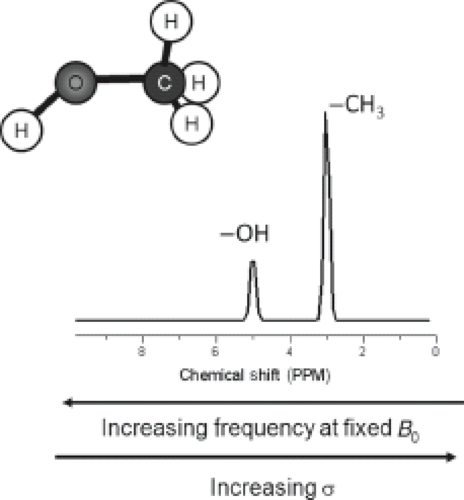 FIGURE 30.1 Representation of a proton spectrum of methanol (CH3OH). The OH hydrogens are less shielded because the oxygen is more electronegative resulting in a higher effective magnetic field (Beff) on the proton and thus has a higher resonance frequency. |
Also note that the ratio of the areas under the two peaks is 3:1 because there are three protons in the CH3 group and one proton in the OH group. The intensity of absorption (the area under the peak) is proportional to the concentration of the nucleus, which is still valid for comparisons between different molecules. This makes NMR spectroscopy a quantitative tool (see Section on “Spectral Quantification”).
J Coupling
Another molecular interaction which modifies the resonance frequency of a spin is known as J coupling (also called indirect dipole–dipole coupling or spin–spin coupling). J coupling results from the interaction between adjacent nuclear spins and is transmitted via the bonding electrons within a molecule. Figure 30.2 illustrates the phenomenon. When spin A of a nucleus is coupled to a spin B, it can “sense” the orientation of that spin in the B0 field. If spin B is aligned with the field, spin A resonates at a frequency different from when spin B is aligned against the field. The population of A spins is, therefore, split into two. Since the probability of finding spin B in a spin-up orientation is the same as the probability of finding it spin down, we observe a doublet for spin A’s resonances with equal intensities. Spin–spin coupling can occur between similar nuclei (homonuclear coupling) or dissimilar nuclei (heteronuclear coupling).
The splitting, J, reflects the strength of local field due to coupling, in Hz, and is independent of the external magnetic field, B0. In addition, when subjected to spin-echo sequences, coupled spins cannot be refocused by a 180-degree pulse if the refocusing pulse acts on both spins, because they always maintain their frequency differences. The result is a phase modulation of the signal that depends on the time delay between the pulses in which the modulation frequency is proportional to 1/J.
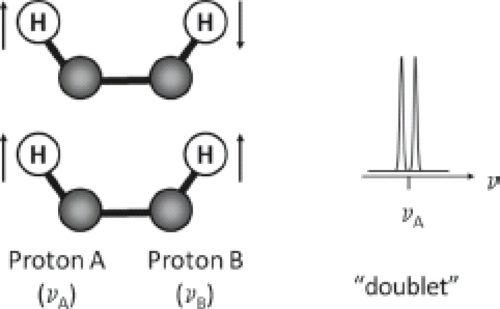 FIGURE 30.2 J coupling between two protons. Proton A and B are coupling partners within the same molecule resonating at different frequencies. When spin B is aligned with the magnetic field, spin A resonates at a frequency different from when spin B is aligned against the field. The population of A spins is, therefore, split into two. Since the probability of finding spin B in a spin-up orientation is the same as the probability of finding it spin down, we observe a doublet for spin A’s resonances with equal intensities. |
Chemical Basis of the In Vivo Brain Mr Spectrum
Major Resonances and Corresponding Metabolites
N-Acetylaspartate (NAA)
In the normal brain, the most prominent spectral peak originates from the trimethylamine group of NAA assigned at 2.02 ppm. NAA is a free amino acid synthesized in neuronal mitochondria by N-acetyl-L-aspartate transferase (1) and it is localized primarily in the central and peripheral nervous systems (2,3), typically at a concentration of 10 to 16 mmol/kg (4,5,6). It has the highest concentration of any water-soluble molecule in the brain and is extremely metabolically active, with 100% turnover in approximately 16 hours (7). The high concentration and rapid turnover rate indicates that this molecule is very important in normal brain metabolism.
Role of NAA in the Nervous System
The function of NAA is not fully understood, but accumulating evidence suggests multiple roles. It is believed to act as a storage form of aspartate and as a precursor of the neurotransmitter N-acetylaspartylglutamate (NAAG), as well as having a variety of other functions (3,8). Additionally, NAA may have a role as a messenger molecule between neurons, astrocytes, oligodendrocytes, and possibly microglia, and has been shown to be an osmoregulator (3,7,9,10). Baslow (9) has proposed that NAA is a key component of a water pump mechanism within the central nervous system (CNS). Having such a mechanism is important, as Baslow has pointed out, because the high metabolic rate of glucose metabolism that occurs in the brain produces a large quantity of water. Without an active mechanism to actively pump water against its gradient, the water production would be deleterious to cellular function. Through the synthesis and degradation of NAA, Baslow has proposed how NAA can serve as a means to enhance the efflux of water from intracellular compartments within the CNS into the blood stream.
Neuropathology of NAA Change
NAA within the adult brain is found almost exclusively in neurons, and serves as a marker of neuronal density and viability (11,12,13,14,15). However, other studies suggested that NAA may be found in mast cells or oligodendrocyte (13,16). Overall, NAA does appear to be a good surrogate marker of neuronal health, but it may sometimes change independent of neuron cell density or function (17): Several quantitative studies of comparing NAA with pathologic measures in human brain tissues have been reported. Cheng et al. (18) found that NAA concentration correlated linearly with neuronal number in a brain from a patient with Pick’s disease. In addition, the same group reported that neuronal counts determined by stereology correlated linearly with the concentration of NAA measured in brain tissue from both Alzheimer’s disease (AD) and control subjects (19). The ratio of NAA to creatine (NAA/Cr) was compared with to a marker of astrogliosis in resected temporal lobe tissues from patients with temporal lobe epilepsy (TLE) by Cohen-Gadol and his coworkers (20). They found a significant inverse relationship of NAA/Cr to the glial fibrillary acidic protein (GFAP) immunoreactivity. This association is not surprising because in this and many other neurologic diseases, neuronal injury occurs along with a gliotic reaction in response to the neurologic insult.
Animal models have been employed to explore the relationship between changes in NAA and corresponding changes revealed by histopathology. In a mouse model Huntington’s disease, Jenkins et al. reported a large (>50%) exponential decrease in NAA with time in both striatum and cortex in mice with trinucleotide (150 CAG, cytosine – adenine guanine) repeats (R6/2 strain). They also reported a linear decrease restricted to striatum in N171–82Q mice with 82 CAG repeats. Both the exponential and linear decreases of NAA were paralleled in time by decreases in neuronal area measured histologically (21,22). In the macaque model of neuroAIDS, Lentz et al. (23) compared levels NAA/Cr with quantitative levels of synaptophysin, microtubule-associated protein 2 (MAP2), and neuron number. They reported that shortly after infection with SIV, the macaque brain had a transient decrease in NAA/Cr. The best correlate of this change was the level of synaptophysin, a measure of synaptic density and synaptodendritic integrity.
Reversible NAA Change
Reversible changes of NAA have been observed, indicating that NAA levels also reflect neuronal dysfunction rather than just neuronal loss. For example, recovery of NAA levels has been observed with reversible ischemia (24) and brain injury (25). Reversal of reduced NAA levels have also been observed with multiple sclerosis (MS) (8), transient ischemia (26,27), and in a macaque model of neuroAIDS (23) in the absence of neuronal loss. It was discovered that during acute infection with SIV, the macaque brain exhibited significant changes in NAA. NAA/Cr best correlated with synaptophysin, a marker of synaptodendritic function. Synaptophysin is a key protein in the formation of synapses and has been shown to decline in a variety of diseases including AD. The best interpretation of this correlation between NAA and synaptophysin suggests that when a neuron experiences a sublethal insult (e.g., ischemia), it responds by reducing the number of synapses, and in parallel, a reduction in the steady-state levels of NAA. Because of this relationship between the synaptic marker and NAA, it is possible that in vivo MRS measurements of NAA not only reflect neuronal number but also the density of viable synapses in the CNS. Interestingly, increased NAA levels have been observed with Canavan’s disease, an inherited disorder in which the enzyme aspartoacylase, involved in the process of degrading NAA to aspartate and acetate, is not being produced, resulting in the accumulation of NAA to toxic levels (8,28).
NAA and NAAG
On clinical MR scanners operating at 1.5 or 3.0 T, the NAA resonance at 2.02 ppm has additional contribution to the signal from NAAG. Using a fully relaxed, short echo time (TE) stimulated echo acquisition mode (STEAM) localization sequence at 2.0 T, separate concentrations for NAA and NAAG were obtained by spectral analysis (LCModel) (29,30). For details on STEAM and point-resolved spectroscopy (PRESS), see Section “Localization Techniques.” With the development of higher magnetic field strength magnets, the separation of NAA and NAAG becomes more feasible.
Total Creatine (Cr)
Another important peak in the proton spectrum is that of creatine, which is assigned at 3.03 ppm. This peak is composed of resonances from creatine (Cr) and phosphocreatine (PCr), and is referred to as total Cr (tCr) or just Cr. Phosphocreatine acts as a high-energy phosphate reservoir for the generation of ATP. Creatine is present in brain, muscle, and blood, and the synthesis of creatine takes place in the kidney and the liver. In vitro, glial cells contain a twofold to fourfold higher concentration of creatine than do neurons (14). Since Cr and PCr are in equilibrium, the tCr peak is commonly assumed to remain stable in size despite bioenergetic abnormalities that occur with many pathologies or with age (31). Consequently, the tCr resonance is often used as an internal standard and is commonly referred to as simply creatine (Cr). However, changes in creatine
have been reported. Since Cr serves as a marker for energy-dependent systems in cells, it tends to be low in processes that have low metabolism, such as in necrosis and infarctions. Furthermore, Cr is typically decreased in brain tumors (32,33,34). However, elevated Cr levels have been reported in patients’ AIDS dementia (35).
have been reported. Since Cr serves as a marker for energy-dependent systems in cells, it tends to be low in processes that have low metabolism, such as in necrosis and infarctions. Furthermore, Cr is typically decreased in brain tumors (32,33,34). However, elevated Cr levels have been reported in patients’ AIDS dementia (35).
Choline-Containing Compounds (Cho)
The choline resonance arises from signals of several soluble components that resonate at 3.2 ppm. This resonance contains contributions primarily from glycerophosphocholine (GPC), phosphocholine (PCho), and choline (Cho). Changes in this resonance are commonly seen with diseases that have alterations in membrane turnover. In diseases such as neoplasms, leukodystrophies, and MS, there is a substantial increase in MRS-visible Cho (36,37,38). The elevated Cho peak reflects a high steady-state level of these molecules that result from increased cellular membrane turnover. Thus, it is increased in most processes that are accompanied by hypercellularity (39,40,41). It is increased in primary and secondary brain tumors with higher Cho/Cr ratios found in malignant tumors (42). Elevated Cho has also been seen in developing brain (43,44) and is also observed in inflammatory and gliotic processes (45,46,47,48,49).
Myo-Inositol (mI)
Myo-inositol is a cyclic sugar alcohol and its most prominent peak is assigned at 3.56 ppm. mI can only be visualized at short TE (e.g., 30 ms). The function of mI is not fully understood, although it is believed to be an essential requirement for cell growth, an osmolyte, and a storage form for glucose (50). mI is primarily located in glia and an increase in mI is commonly thought to be a marker of gliosis (51). The identification of mI can be important in the evaluation of brain tumors (32,52). This metabolite is usually decreased in high-grade primary brain tumors, but visible in low-grade neoplasms (53). Elevated mI levels have been associated with AD (54,55,56), AIDS dementia, other neurodegenerative diseases, and brain injury (57). In addition, elevated mI has been reported in newborns (43). Reduced mI is observed in hepatic encephalopathy (58).
Glutamate (Glu) and Glutamine (Gln)
Glutamate (Glu) is the major excitatory neurotransmitter of the brain, although it has other important metabolic functions (4,50,59). Excess of glutamate surrounding neural cells can be toxic and can cause neuronal death. Cerebral glutamate concentration is reported to be increased in cerebral ischemia (60), hepatic encephalopathy (61), and Reye’s syndrome (62).
The amino acid glutamine is a precursor and storage form of glutamate and is primarily located in astrocytes. Glutamate and glutamine have strongly coupled spin systems that give rise to complex spectra (63,64). Since glutamine and glutamate are structurally very similar, it is very difficult to separate their resonances at low field strength, and therefore, the sum of Glu and Gln is commonly referred to as Glx. The peaks of interest resonate between 2.1 and 2.5 ppm (left shoulder of NAA). While it is possible to quantify Glu and Gln independently at lower field strengths, e.g., 3 T (65), these overlapping peaks might be more reliably resolved at higher field strengths (66,67).
Lactate (Lac)
Under normal conditions, the lactate concentration is very low in the adult brain. This resonance (observed as a doublet) occurs at 1.32 ppm. Confirmation of the presence of lactate can be achieved by obtaining MRS with a TE of 144 ms, which results in the inversion of the lactate doublet below the baseline or with a TE of 288 ms resulting in MR spectra in which the lipid peaks have typically decayed due to T2 effects. Lactate is produced by anaerobic metabolism and has been detected in stroke patients (68,69,70). It has been reported that lactate levels after acute stroke correlate strongly with apparent diffusion coefficient (ADC) values (27). Increased lactate has been found during hypoxia (71), mitochondrial diseases (72,73,74), seizures (75), and in the first hours after birth (76).
The presence of lactate in brain tumors has received a great deal of attention. This situation occurs in highly cellular and metabolic lesions that outgrow their blood supply. The presence of lactate indirectly measures glucose utilization. Increased energy demands by highly cellular lesions lead to excessive oxygen utilization, and increased reliance on anaerobic glycolysis resulting in the production of lactate. Therefore, the presence of lactate often accompanies malignant neoplasms (77). It has been observed that regions containing lactate correspond to areas of increased cerebral blood volume (CBV) in brain perfusion studies and thus may serve as an indicator of angiogenesis, another feature typical of highly malignant brain tumors (78).
Lipids (Lip)
MRS obtained with short TE offers the possibility of visualizing additional resonances, particularly those produced by compounds having short relaxation times such as lipids. Lipids resonate between 0.8 and 1.5 ppm and may obscure the presence of lactate. Mobile lipids are generally found in necrosis and, as such, are indicators of high-grade malignancies, both primary brain tumors and metastases (79,80). Alternatively, elevated lipids are an indicator for radiation necrosis. Radiologists reading MR spectra should use caution when interpreting lipid signals as lipids may also be present in the spectra due to contamination by subcutaneous fat and fat from marrow of the skull.
Minor Resonances and Corresponding Biochemicals
γ-Aminobutyric Acid (GABA)
γ-aminobutyric acid (GABA) is an amino acid and an inhibitory neurotransmitter. GABA concentrations in the brain are close to the detection limits of in vivo MRS. In addition, the GABA resonances overlap considerably with contributions from other more abundant metabolites, in particular, creatine. However, the invention of specialized MRS techniques, such as selective editing techniques (81,82), localized two-dimensional (2D) chemical shift methods (83), or multi-quantum filtering methods (84), has enhanced the ability to detect and measure GABA. Proton MRS studies have found reduced or abnormal GABA concentrations in several neuropsychiatric disorders, including epilepsy, anxiety disorders, major depression, drug addiction (85), and autism (86).
Glutathione (GSH)
Glutathione is a tripeptide made up of glycine, cysteine, and glutamate; it exists in a reduced (GSH) and oxidized (GSSH) form in which GSH is an antioxidant. GSH is primarily located in astrocytes at a concentration of 2 to 3 mmol/kg and essential for maintaining normal red-cell structure, keeping hemoglobin in the ferrous state, serves in an amino acid transport system, and is a storage form of cysteine. The resonances of GSH overlap with those of Glu, Gln, GABA, Cr, and NAA; however, double quantum coherence filtering technique enables the selective
observation of the resonances at 2.9 ppm from the overlapping resonances of GABA, creatine, and aspartate. Decreased GSH levels have been observed in patients with ALS (87), bipolar disorder (88), and major depression (89).
observation of the resonances at 2.9 ppm from the overlapping resonances of GABA, creatine, and aspartate. Decreased GSH levels have been observed in patients with ALS (87), bipolar disorder (88), and major depression (89).
Glycine (Gly)
Glycine is an amino acid that acts as an inhibitory neurotransmitter and antioxidant, and is distributed throughout the CNS. Elevated glycine has been reported in tumors (90) and in patients with hyperglycinemia (91). For in vivo MRS measurements, the glycine resonance overlaps with those of mI (at 3.55 ppm), making definite observation of glycine not possible at shorter TEs, although its presence may be verified at longer TEs due to the reduction of the inositol multiplet.
Alanine (Ala)
Another metabolite that may be of interest when performing MRS of intracranial tumors is alanine. It is a nonessential amino acid that resonates between 1.3 and 1.4 ppm, and may be overshadowed by the presence of lactate and lipids. Alanine has been found to be elevated in some meningiomas (32).
Valine (Val)
Valine is an essential amino acid necessary for protein synthesis. The spectrum consists of two doublets from the two methyl protons that overlap with resonances of leucine and isoleucine in the range of 0.95 to 1.05 ppm. Hypervalinemia and branched-chain ketonuria are some of the diseases in which valine levels become elevated (92). Increased concentrations have also been observed in brain abscesses (93). Furthermore, accumulation of the branched-chain amino acids including valine, leucine, and isoleucine can be detected neonates with maple syrup urine disease (MSUD), a disorder caused by a deficiency of the branched-chain α-ketoacid dehydrogenase enzyme complex (Table 30.2) (94).
Other Amino Acids
Macromolecules
Like lipids, macromolecules can only be visualized at short TEs (124). The presence of pathologically altered macromolecules or mobile lipids may provide useful additional diagnostic information in various pathologies, such as brain tumors and MS (125,126).
Table 30.3 summarizes the key metabolites, including their major resonance and the associated changes with brain disease.
TABLE 30.2 Variations of Major 1H MRS Metabolites in Selected Inborn Errors of Metabolism | ||||||||||||||||||||||||
|---|---|---|---|---|---|---|---|---|---|---|---|---|---|---|---|---|---|---|---|---|---|---|---|---|
| ||||||||||||||||||||||||
TABLE 30.3 Summary of the Key Metabolites, Including Their Major Resonance and the Associated Changes with Brain Disease | ||||||||||||||||||||||||||||||||||||||||||||||||||||||||
|---|---|---|---|---|---|---|---|---|---|---|---|---|---|---|---|---|---|---|---|---|---|---|---|---|---|---|---|---|---|---|---|---|---|---|---|---|---|---|---|---|---|---|---|---|---|---|---|---|---|---|---|---|---|---|---|---|
| ||||||||||||||||||||||||||||||||||||||||||||||||||||||||
In Vivo Magnetic Resonance Spectroscopy
The basic principles described in the previous section were primarily based on ex vivo samples using an NMR spectrometer. Figure 30.3A shows a typical NMR spectrum of human brain extract measured with a 14 T (600 MHz) NMR spectrometer. However, to be clinically relevant, MRS needs to be performed in vivo. Unfortunately, the spectral quality is compromised by magnetic field inhomogeneity and usually low field strengths. In vivo spectra are further broadened by chemical shift anisotropy, dipolar coupling from motionally constrained species, as well as magnetic susceptibility variations in the tissue, resulting in a loss of biochemical information. However, in many cases the spectral quality is still sufficient to diagnose diseases, monitor treatments, or to help understand the pathogenesis of diseases. Figure 30.3B shows a typical proton MR spectrum from the white matter (WM) of the centrum semiovale of a human brain acquired at a short TE of 35 ms at 3.0 T. The most prominent peak arises from NAA at 2.0 ppm. The other major peaks include creatine (Cr) and choline-containing compounds (Cho) and are observed at 3.0 and 3.2 ppm, respectively. Cr and Cho both have approximately half the height of NAA in the centrum semiovale of normal controls. The next section discusses metabolites and their significance for diagnosis.
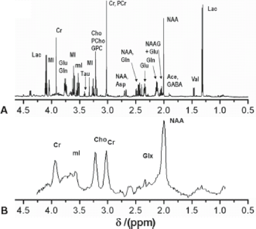 FIGURE 30.3 Comparison between ex vivo NMR and in vivo MRS. A: Typical ex vivo NMR spectrum of human white matter brain extracts measured with a 14 T (600 MHz) NMR spectrometer using a single pulse sequence with TR 20 s and 64 acquisitions. B: Typical proton MR spectrum from the white matter semiovale of a healthy male subject acquired with a single voxel PRESS sequence (TR/TE = 2,300/30, NS = 160) at a 3.0-T MRI scanner. |
Localization Techniques
For diagnostic purposes one is interested in directly comparing spectra from pathologic or abnormal tissue with normal tissue. Thus, to measure MR spectra in vivo, one has to be able to define the spatial origin of the detected signal. (A) Single-voxel spectroscopy (SVS) uses selective excitation pulses to localize a voxel of typically 3 to 8 cm3. SVS has the advantage of higher SNR and typically shorter acquisition times. However, the additional scan time typically permits acquisition of only a few locations. (B) Magnetic resonance spectroscopic imaging (MRSI) can be obtained in two or three dimensions. MRSI allows one to collect the spectral information from a volume consisting of many voxels with individual voxel sizes of typically 0.5 to 3 cm3 and makes it possible to cover large brain areas. However, spectra typically have a lower SNR compared to SVS.
Single-Voxel Spectroscopy
Localization of protons in a 3D volume requires the application of three distinct magnetic gradients during the pulse sequence. The two most commonly used localization methods include STEAM (127) and PRESS (128). In both sequences, three selective pulses along with three orthogonal gradients generate a stimulated-echo or a spin-echo within the volume of interest or voxel: (i) STEAM uses three consecutive slice selective 90-degree pulses that create a stimulated echo from the VOI; (ii) PRESS uses a selective 90-degree pulse followed by two slice-selective 180-degree pulses that create a spin echo. Both sequences have been compared in detail by Moonen et al. (129).
STEAM provides excellent slice selection profiles because frequency selective 90-degree pulses generally have a good slice profile, and thus allows for sampling of smaller VOIs. In addition, signal losses due to T2 relaxation remain minor as the magnetization is stored on the z-axis between the second and third selection pulses. Therefore, STEAM is able to utilize very short TEs and it permits visualization of metabolites with shorter TEs such as mI, glutamate, and glutamine. Excellent water suppression can be achieved because additional water suppression pulses can be applied during the mixing time when the magnetization is stored in the z-axis. However, the stimulated echo has an intrinsically lower (50%) signal compared to MRS exams obtained with PRESS sequence, which leads to a lower SNR or longer scan times. PRESS typically requires a longer TE and consequently the signal from most metabolites in the brain would decay, except those of Cho, Cr, NAA, and Lac. In recent years, however, PRESS can be performed using short TEs, for example, 30 ms, which has made it the most commonly used technique in clinical MRS.
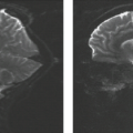
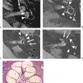
In vivo MRS at higher field strengths is associated with (i) chemical shift displacement errors, (ii) spatial nonuniformity of RF excitation, and (iii) contamination with subcutaneous lipid signal. To address these problems, adiabatic pulses have been implemented in techniques such as LASER (130,131) and semi-LASER (132,133). The most commonly used adiabatic pulse is the hyperbolic secant adiabatic full passage (AFP) inversion pulse and the hyperbolic secant adiabatic half passage (AHP) pulse to archive a 90-degree pulse (134). Figure 30.4 compares spectra acquired with a PRESS and a LASER sequence in a tumor patient.
Magnetic Resonance Spectroscopic Imaging
MRSI, or chemical shift imaging (CSI), allows one to collect the spectral information from a volume consisting of many voxels. Like MRI, it produces an image of an object, but now each pixel also contains the spectral information. MRSI is superior for many clinical studies when it is necessary to obtain metabolic information of a large or heterogeneous lesion—possibly revealing new tumor growth that is not yet visible on a regular MRI. Additionally, spectral information from control regions may be obtained simultaneously.
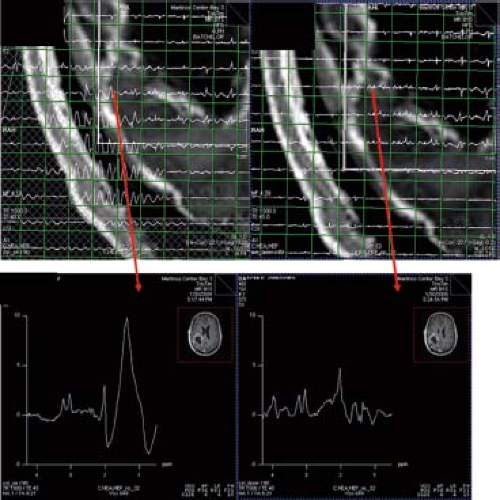 FIGURE 30.4 Comparison between spectra in a tumor patient acquired with a PRESS (left) and a LASER sequence (right). (Red arrows) are pointing to the magnified voxels below. The PRESS sequence has been acquired with outer volume suppression (OVS), yet one can detect large lipid artifacts from skull inside the VOI. Using a LASER sequence (w/o OVS) these artifacts are mitigated. (Courtesy: Ovidiu Androresi and Greg Sorensen.) |
The MRSI sequence is similar to an imaging sequence; however, the major difference is that no readout or frequency-encoding gradient is applied during data collection, because high magnetic field homogeneity is necessary during data acquisition to obtain the narrow line widths essential in MRS. Localization in spectroscopy is implemented with slab excitation followed by phase encoding (PE) gradients. The data can then either be displayed as a grid of many voxels, as individual voxels, or as metabolite maps in which the intensities displayed in the image are proportional to a particular metabolite signal strength (Fig. 30.5).
Fast MRSI Techniques
The main limitation of MRSI is the lengthy acquisition times, especially with 3D data acquisition. A number of fast CSI experiments have been presented, that promise to significantly reduce data acquisition duration. Some improvement may be achieved by acquiring data by reduced k-space sampling. Circular k-space sampling reduces the encoding time by 22% as compared to traditional square or rectangular sampling (135). When multiple averages are acquired, weighted k-space sampling reduces signal averaging of higher k-space. Comparison of k-space sampling schemes for multidimensional MRSI can be found at Hugg et al. (136).
Fast CSI concepts have evolved from concepts related to spatial encoding using gradient switching during acquisition (137,138). These techniques were further developed by others (139,140,141). They work based on the fact that the dwell time to encode spectral information is long due to the relatively small spectral window—approximately 1 ms while the time to encode the spatial information is usually much faster—tens of microseconds. Therefore, it is possible to encode spectral and spatial information in an interleaved fashion using a series of inverted readout gradients that generates a series of echoes. Those interleaved spatial–spectral encoding methods can be either echo-planar imaging (EPI) (137) or spiral based.
 FIGURE 30.5 MRSI data can either be displayed as a grid of many voxels or as metabolite maps in which the intensities displayed in the image are proportional to a particular metabolite signal strength. In this example, the red indicates high concentration of choline that co-localizes with the contrast-enhancing mass lesion. |
The proton echo-planar spectroscopic imaging (PEPSI) sequence can be based on either STEAM or PRESS; it uses standard phase encoding (PE) in the x-direction, while PE in the y-direction is replaced by bipolar gradients, switching during data acquisition (141).
Spiral trajectories in k-space allow even faster encoding of spatial information due to faster gradient duty cycle (142,143). In spiral imaging, k-space is filled by spiral readouts that are produced by sinusoidally varying gradients in both the x– and y-axes. Recently, Andronesi et al. (144) implemented a 3D volumetric in vivo MRSI sequence using spiral trajectories and compared spectra acquired with a conventional PE sequence (1 cm3 voxels) with spectra acquired with the spiral encoding at similar and higher spatial resolution (0.39 cm3 voxels) and with shorter imaging time. 3D MR spectroscopic images were acquired 4× faster with spiral protocols than with the elliptical PE protocol at low spatial resolution (1 cm3). Higher–spatial resolution images (0.39 cm3) were acquired twice as fast with spiral protocols compared with the low–spatial resolution elliptical PE protocol. These improvements in image quality and imaging time allow more routine acquisition of spectroscopic data in the clinical setting (Fig. 30.6).
Sensitivity encoding (SENSE) or simultaneous acquisition of spatial harmonics (SMASH) offers a new, highly effective approach to reducing the acquisition time in spectroscopic imaging. Phased array RF coils increase sensitivity especially in the cortical areas compared to conventional head coils. Compared to conventional fast CSI techniques, this method permits a reduction in the number of PE steps in each PE dimension. Fourfold reduction of scan time is achieved at preserved spectral and spatial resolution, maintaining a reasonable SNR (145,146).
Another more time-efficient way to sample the third spatial dimension can be achieved with a 3D hybrid of 2D CSI and 1D fourth-order Hadamard spectroscopic imaging (HSI) sequence (147,148). CSI using PE with Fourier transformation methods suffers from two disadvantages: the field of view (FOV) needs to be larger than object to prevent aliasing extraneous signal and the spectral contamination from outside the voxel. The effect of the localization error or “voxel bleed” is reduced with increasing resolution. Thus, in a case where there are only a few partitions, for example, four in z-direction, Hadamard encoding is superior to CSI in the accuracy of localization.
Water and Fat Suppression
Brain metabolite concentrations are on the order of 10 millimolar (mM) or less compared with the ∼80 M concentration of water protons (149). Additionally, the extremely large lipids within skull, marrow, and extra cranial fat are also present in high concentrations (150). Therefore, it is essential to suppress the water and the lipid peaks to reliably measure the metabolite contractions. Water suppression can be accomplished by chemical selective saturation (CHESS) pulse on the water signal at 4.7 ppm (151), thereby suppressing the water signal 1,000- to 10,000-fold. The residual water may then be used as internal reference for phasing and frequency correction.
The suppression efficiency in CHESS is affected by T1 relaxation and RF-pulse flip angles (which depend on B1) and sequence timing. Ogg et al. (152) introduced a water suppression scheme that is independent of B1 and T1, called WET (water suppression enhanced through T1 effects). This method uses four frequency-selective RF pulses with different numerically optimized flip angles and thus producing better water
suppression without time-consuming optimization prior to each measurement.
suppression without time-consuming optimization prior to each measurement.
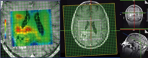 FIGURE 30.6 3D laser spiral MRSI. The fast spiral readout allows full 3D tumor sampling in approximately 7 minutes while maintaining high resolution (0.7 × 0.7 × 0.7 cm3 = 0.34 cm3) and an acceptable signal-to-noise ratio (SNR) (144). |
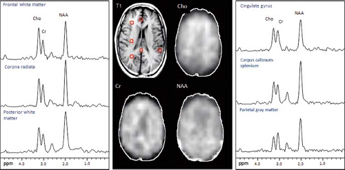 FIGURE 30.7 MRSI data recorded using multi-slice MRSI pulse sequence with CHESS water suppression and outer volume saturation band lipid suppression. Metabolite images of Cho, Cr, and NAA from one slide of the level of the lateral ventricles in a normal volunteer (52-year-old white male). Scan parameters were TR 2,300 TE 280, 32 × 32 matrix, 4 slices (only 1 shown), 15 mm thick, nominal voxel size 0.8 cc. NAA is fairly evenly distributed at this level while choline shows an increase from posterior to anterior brain regions. (Courtesy of Dr. Peter Barker, Johns Hopkins University School of Medicine, Baltimore, MD.) |
Lipids may be avoided by placing the VOI completely inside the brain excluding skull to avoid signal from marrow and subcutaneous fat. Additionally, or as an alternative, outer volume suppression (OVS) pulses are used for further lipid suppression (153). An inversion pulse scan can also be used for lipid suppression (154), taking advantage of the fact that T1 relaxation times of most metabolites vary between 1,000 and 2,000 ms while spin–lattice relaxation time of lipids are much shorter (approximately 300 ms). Figure 30.7 illustrates typical MRSI data recorded using eight OVS pulses arranged in an octagon on axial slides in order to saturate as much pericranial lipids as possible while the signal from the brain is unperturbed (153).
Acquisition Parameters
As with MRI, the choice of TE and repetition time (TR) can have an enormous effect on the appearance of the information obtained in a proton MRS study. MR spectra obtained with shorter TEs (∼30 ms) allow the detection of more metabolites including glutamate, glutamine, and mI. However, the baseline is typically more complicated due to increased lipid and macromolecular background signals. Spectra obtained with longer TEs (144 or 288 ms) depict reduced number of metabolites. But, spectra are easier to process and analyze due to the relatively flat baseline (Fig. 30.8). In addition, lactate (1.3 ppm) and alanine (1.5 ppm) doublets are inverted, thereby allowing better differentiation between these metabolites and lipids/macromolecules.
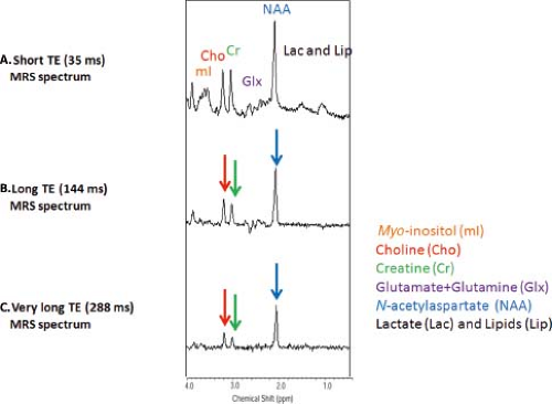 FIGURE 30.8 Effect of TE. Top: Proton MR spectrum obtained at short echo time (TE = 35 ms). Middle: MR spectrum obtained at intermediate echo time (TE = 144 ms). Bottom: MR spectrum obtained at long echo time (TE/TR = 288 ms). All spectra were acquired at 3 T with a single-voxel PRESS sequence from the parietal gray matter with 128 acquisitions, TR 1,500 ms. |
Spin–lattice relaxation times for selected resonances at 1.5 T vary between 1,100 and 1,700 ms (155). Ideally, one has to wait three times T1 (3 × 1,500 ms = 4,500 seconds) to gain approximately 95% of the original magnetization. With longer TR (>3 seconds), the SNR and the quantification improve. However, a long TR results in a long exam time. Therefore, typical TRs for clinical MRS experiments lie between 1 and 3 seconds.
Field Strength
Unfortunately, MRS suffers from inherently low SNR resulting in MRSI with low spatial resolution because the targeted metabolites are dilute. MRS SNR can be improved significantly by using higher magnetic field strengths since the SNR is proportional to B0, according to Equation (6):
with Nv being the number of spins and T the temperature.
Figure 30.9A shows the spectra from the parietal cortex obtained at three different field strengths, 1.5, 3.0, and 7 T of a healthy nonhuman primate. The SNR becomes higher at higher fields. The increased chemical shift dispersion at 7 T results in greater separation of the resonance peaks, and as a consequence, allows for better quantification of those metabolites that generally overlap with others such as glutamate and glutamine (collectively called Glx) and mI. Figure 30.9B shows a 7-T spectrum of the parietal cortex obtained using a STEAM (TE = 20 ms) sequence with a transverse electromagnetic (TEM) head coil optimized for macaque studies. Improvements in spectral resolutions are evident. Excellent resolution in in vivo 1H NMR spectroscopy of human brain at 7 T has been reported using ultra-short echo-time STEAM sequences (67).
Editing Techniques
Splitting of resonance lines into multiplets due to J-modulation results in signal loss and cancellation, and can make the quantification of an MR spectrum more challenging (157,158). In addition, many resonances of similar frequencies in the proton MR spectrum overlap. To overcome overlap, there are two major strategies for spectral editing in vivo. One method is based on difference spectroscopy and editing the other one on multiple quantum filtering.
In difference editing, a selective and nonselective spin-echo spectra are acquired; the difference spectrum contains the target metabolite signal while all other contributors will be nulled (159,160).
For the detection of GABA, the MEGA-PRESS (MEshcher–GArwood Point RESolved Spectroscopy) sequence (82) is currently the most widely used MRS technique (161). The sequence involves the collection of two interleaved datasets: In one dataset, an editing pulse is applied to GABA spins at 1.9 ppm in order to selectively refocus the evolution of J-coupling to the GABA spins at 3 ppm (often referred to as ‘ON’). In the other, the inversion pulse is applied at 7.5 ppm so that the J-coupling evolves freely throughout the TE (often referred to as ‘OFF’). Subtraction of the nonrefocused OFF spectrum from the refocused ON spectrum retains only those peaks that are affected by the editing pulses. Thus, in vivo, the edited spectrum contains
signals close to 1.9 ppm (those directly affected by the pulses), the GABA signal at 3 ppm (coupled to GABA spins at 1.9 ppm), the combined glutamate/ glutamine (Glx) peaks at 3.75 ppm (coupled to the Glx resonances at approximately 2.1 ppm), and J-coupled macromolecular (MM) peaks. Figure 30.10 shows two GABA-edited spectra acquired from the parietal lobe of a healthy 9-year-old boy. Multiple quantum filtering can be done in just one sequence, exploiting the difference between coupled and uncoupled metabolites (162).
signals close to 1.9 ppm (those directly affected by the pulses), the GABA signal at 3 ppm (coupled to GABA spins at 1.9 ppm), the combined glutamate/ glutamine (Glx) peaks at 3.75 ppm (coupled to the Glx resonances at approximately 2.1 ppm), and J-coupled macromolecular (MM) peaks. Figure 30.10 shows two GABA-edited spectra acquired from the parietal lobe of a healthy 9-year-old boy. Multiple quantum filtering can be done in just one sequence, exploiting the difference between coupled and uncoupled metabolites (162).
 FIGURE 30.9 Effect of FIELD STRENGTH. A: Single-voxel 1H MRS spectra from the parietal cortex of rhesus macaques obtained at three different field strengths, 1.5 T (left), 3.0 T (middle), and 7 T (right). Increasing magnet field strength produces an approximately linear increase in the signal-to-noise ratio. B: Single-voxel 1H MRS STEAM spectrum from the parietal cortex obtained of a rhesus macaque at 7 T. High field strength also improves spectral dispersion. For example, the glutamate and glutamine resonances at 2.35 and 2.45 ppm were clearly separated. In addition, we could detect J coupling between the CH2 protons of myo-inositol. Acquisition parameters include TE = 15 ms, TR = 3000 ms, VOI 1.2 × 1.2 × 1.2 cm3, 196 acquisitions. (Adapted from Ratai EM, Pilkenton S, He J, et al. CD8 +lymphocyte depletion without SIV infection does not produce metabolic changes or pathological abnormalities in the rhesus macaque brain. J Med Primatol 2011;40(5):300–309.) |
 FIGURE 30.10 GABA edited spectrum acquired from a 3 × 3 × 3 cm3 ROI centered in the precuneus region in a healthy 9-year-old boy. For the detection of GABA, the MEGA-PRESS (MEshcher–GArwood Point RESolved Spectroscopy) sequence (82) has been used. Data were acquired at 3 T using a 32-channel receiver coil. Data parameters: TE/TR = 68 ms/1,500 ms, spectral width = 2 kHz and 160 acquisitions (8 minutes). |
Regional Variations
Regional differences in metabolite concentrations occur throughout the brain. There are differences between white and gray matter (GM), as well as between cerebrum, cerebellum, brainstem, and deep gray structures (Fig. 30.11). Moreover, there are differences between individuals. To properly evaluate a disease process in the brain, it is best to compare spectra from the voxel of interest to one from a similar location in a normal brain. In the case of the cerebrum, comparison with a voxel localized to a similar location within the contralateral hemisphere is appropriate.
Spectral Quantification
There are longstanding discussions and disputes on the best way to quantify MRS signals, specifically relative versus absolute quantification. The total area under the metabolite resonance peak is proportional to the concentration of that specific metabolite and the integration of this area is primary task needed for quantification. The easiest method is to employ metabolite ratios such as NAA/Cr or Cho/NAA. Ratios reported using creatine as an internal standard is often based on the assumption that the Cr concentration does not change during the disease process which is sometimes, but not always true. Alternatives include ratios of each metabolite of interest to the sum of metabolites, or using the spectral information from normal brain as a reference. Ratios are relatively easy to determine and are more reproducible than absolute concentration determination. However, when a change is detected, it may not be possible to determine whether it is due to a change in the numerator, denominator, or both. Absolute quantification of brain metabolites by MRS is more difficult, and they are generally expressed in units of mmol/kg.
Methods used for absolute quantification include (a) phantom replacement techniques in which the in vivo metabolite concentrations will be estimated from the ratio of the in vivo and phantom signals, with corrections for differences in T1 and T2 relaxation times, RF coil loading, and receiver gain (163,164,165,166), (b) the use of unsuppressed water signal as a reference (167,168,169); (c) the use of an external reference (170,171), and (d) reciprocity (172).
To date automated parametric spectral analysis methods have been implemented to quantify metabolite concentrations. These methods seek to determine the optimum parameters that enable some functions (so-called model functions) to best
describe the MRS data. These model functions are based on prior information. Fortunately, considerable information on the observable metabolites and their spectral characteristics are available (4). Parametric modeling based on a priori spectral information has been made reasonably robust (30,173,174,175,176,177). Spectral fitting can be done in the time (178) or frequency domain (179). Currently, the most commonly used MRS analysis programs are LCModel (30,180,181) and jMRUI (182,183).
describe the MRS data. These model functions are based on prior information. Fortunately, considerable information on the observable metabolites and their spectral characteristics are available (4). Parametric modeling based on a priori spectral information has been made reasonably robust (30,173,174,175,176,177). Spectral fitting can be done in the time (178) or frequency domain (179). Currently, the most commonly used MRS analysis programs are LCModel (30,180,181) and jMRUI (182,183).
 FIGURE 30.11 MRS regional variations in normal adult brain. 1H MRS spectra are shown of a 30-year-old female adult brain from white matter (WM), gray matter (GM), basal ganglia (BG), and cerebellum (CB) using an 8-cc voxel, TR/TE = 2,300/30 and 160 averages at 1.5 T. |
Limitations of Clinical MRS
A major limitation associated with in vivo MRS is due to the low SNR resulting in coarse spatial resolution; however, there are others. We will identify a few of the more important.
B0 Inhomogeneities
MRS is very sensitive to magnetic field (B0) inhomogeneities that cause broad line widths. This can result in peak overlap and poor quantification. Therefore, shimming to optimize B0 homogeneity at the beginning of each spectral acquisition is mandatory, in order to obtain narrow line widths in the MR spectrum. To minimize B0 inhomogeneities, a shimming procedure is used for both MRS and MRI. The MR instrument uses several additional coils that produce static magnetic field gradients designed to correct the existing field inhomogeneity.
Voxel Location
Proximity of the VOI to the paranasal sinuses and mastoids can result in line broadening and susceptibility artifacts. Additionally, iron and minerals that accumulate in the basal ganglia cause susceptibility broadening, resulting typically in lower-quality spectra. As previously stated, proximity of the VOI to scalp can result in contaminating lipid signals. However, techniques to suppress lipid signals can minimize this problem. There are limitations to the spatial selectivity of the MR spectrum. The spectrum for any given voxel contains contribution from neighboring voxels because the point-spread function is not an ideal cube (184).
B1 Inhomogeneities
MRI, MRS is also subject to chemical shift artifacts. The chemical shift between NAA and choline nuclei is about 1.3 ppm (∼85 Hz at 1.5 T, ∼250 Hz at 3 T, and 450 Hz at 7 T). Because of this difference in resonance frequency between NAA and Cho protons, spatial misregistration takes place when converting the MR signals from the frequency to the spatial domain by the Fourier transformation. To minimize these, saturation bands positioned outside the visible VOI have been employed. In addition, there is a focus to using adiabatic pulses to compensate for RF inhomogeneity and reduce the chemical shift displacement error (131,185).
Motion Artifacts
Poor patient cooperation resulting in motion artifacts often limits the feasibility of MRI and MRS. Anesthesia is not always feasible and, in addition, carries risks to the patients (102). Thus motion-corrected sequences have been employed that may allow for the reduction in the need for sedation. Using new techniques such as propeller MRI, it has become possible to oversample k-space and thereby compensate for motion and allow follow-up MRI without sedation (186,187). As alternative to retrospective motion-corrected techniques, it is also possible to prospectively correct motion. Using image-based navigators, it is possible to correct motion in structural imaging, single-voxel and multivoxel spectroscopy prospectively (188,189,190,191,192,193,194).
Reproducibility
In clinical studies, reproducible measurements of metabolite concentrations are of paramount importance for detecting the effect of the disease or treatment in an individual or in a group. Several studies have been performed on the reproducibility of quantitative MRS of the human brain using SVS (195,196,197,198,199) and spectroscopic imaging methods (200,201,202). While intra-individual CVs for single-voxel MRS were reported to vary between 3.3% and 8.1% for absolute quantification (196), reproducibility of metabolite ratios obtained with MRSI was somewhat poorer. Importantly, standard clinical hardware generates reproducible MRS data from the human brain in a multicenter setting provided that identical and optimized acquisition protocols and calibration schemes are used (Fig. 30.12).
The following summarizes the technical factors necessary for a clinically interpretable MR spectrum of the brain:
Spectrum SNR >3 for major resonances
Spectral resolution: full width at half maximum (FWHM) of metabolites <0.1 ppm
Line shape: symmetric
Water suppression >98%
No lipid contamination from the scalp
Artifacts such as chemical shift artifact, ghosting, patient motion, eddy currents, and volume averaging are absent or minor.
Details on these technical criteria can be found in the following paragraphs and in a comprehensive review by Kreis et al. (204):
Nonproton MRS
MRS can be performed using nuclei other than 1H such as 13C, 19F, 31P, etc. 1H is most commonly used because it has the highest sensitivity compared to the other nuclei, and 1H MRS is easy
to perform as we can use the same RF coils that are also used for standard MRI.
to perform as we can use the same RF coils that are also used for standard MRI.
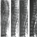
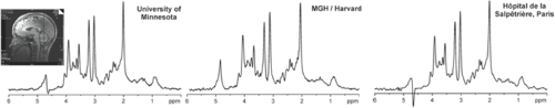 FIGURE 30.12 Reproducible high MR spectral quality from multiple sites. 1H MR spectra were acquired at three different sites from cerebellar volume of interest (10 × 25 × 25 mm3, as shown on T1-weighted midsagittal image) in three healthy individuals. Spectra were obtained with 3.0-T MR units with same acquisition protocol (fast automatic shimming technique by mapping along projections, or FASTMAP, semi-LASER [localization by adiabatic selective refocusing] (203), 5,000/28, 64 repetitions). (Spectra from the Center for Magnetic Resonance Research, University of Minnesota; courtesy of Gülin Öz, MGH = Massachusetts General Hospital and Hôpital de la Salpêtrière courtesy of Fanny Mochel, MD, PhD) (Adapted from Oz G, Alger JR, Barker PB, et al. Clinical proton MR spectroscopy in central nervous system disorders. Radiology 2013;270(3):658–679, with permission.) |
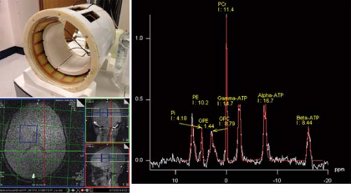 FIGURE 30.13 2D 31P CSI spectra of the brain of a healthy 10-year-old boy. Data were acquired with a 3.0-T MR unit using an 8-channel receive 31P coil and 31P birdcage transmit coil. Localization was confirmed using the 1H body coil. MRS data were acquired using a CSI-FID sequence with TR 1,500 ms, 32 averages, and 8 × 8 phase-encoding steps. |
31P MRS is informative on cellular bioenergetics because it can measure adenosine triphosphate (ATP) and phosphocreatine (PCr). It may also be used to measure phosphodiester compounds (PDEs), inorganic phosphate (Pi), and phosphomonoester compounds (PMEs). The chemical shift of the Pi peak is pH dependent and is commonly used for in vivo measurement of intracellular pH. Phosphorus has a larger chemical shift range (approximately 25 ppm) than protons (approximately 10 ppm). Solvent, for example, water suppression schemes are not required for 31P MRS; however, the strength of the MR signal is approximately an order of magnitude lower than those from protons. Thus, lower spatial resolution and/or longer exam times are required in 31P MRS to achieve adequate SNR. Despite these limitations, 31P has successfully been employed in brain (184,205,206,207,208,209,210,211,212,213), muscle (214,215,216), liver (217,218), heart (219,220,221,222), kidney (223,224), and prostate (225), as well as other regions (Fig. 30.13).
Related posts:
Stay updated, free articles. Join our Telegram channel

Full access? Get Clinical Tree


