Magnetic resonance (MR) imaging is the method of choice to evaluate the cranial nerves. Although the skull base foramina can be seen on CT, the nerves themselves can only be visualized in detail on MR. To see the different segments of nerves I to XII, the right sequences must be used. Detailed clinical information is needed by the radiologist so that a tailored MR study can be performed. In this article, MR principles for imaging of the cranial nerves are discussed. The basic anatomy of the cranial nerves and the cranial nerve nuclei as well as their central connections are discussed and illustrated briefly. The emphasis is on less known or more advanced extra-axial anatomy, illustrated with high-resolution MR images.
Magnetic resonance (MR) imaging is the method of choice to evaluate the cranial nerves. Although the skull base foramina can be seen on CT, the nerves themselves can only be visualized in detail on MR. To see the different segments of nerves I to XII, the right sequences must be used. It goes without saying that detailed clinical information is needed by the radiologist so that a tailored MR study can be performed. In this article, the MR principles for imaging of the cranial nerves are discussed. The anatomy of the 12 cranial nerves will be addressed but it is not possible to describe all of the anatomy in one article. Therefore, the basic anatomy of the cranial nerves and the cranial nerve nuclei as well as their central connections are discussed and illustrated briefly while the emphasis is on less known or more advanced extra-axial anatomy, illustrated with high-resolution MR images. For more complete anatomic descriptions and anatomic and/or MR illustrations the reader is referred to dedicated already existing complete works.
MR technique
The MR technique must be pushed to its limits to see all 12 cranial nerves and especially some of the segments or branches of these nerves that are more difficult to depict. Imaging plane, coil and sequence choice, slice thickness and in-plane resolution, use of special techniques like parallel imaging, asymmetric k-space, fat suppression, and so forth will all influence the final image quality.
Imaging Plane
All cranial nerves are paired and therefore it is wise to compare size and signal intensity of both nerves. The coronal plane is best suited to study the cranial nerves I to VI, as they have a dominant postero-anterior course. Cranial nerves VII to XII run in an antero-lateral-caudal direction but the lateral component is dominant. Hence the best plane will be the axial plane. Nevertheless it is always safe to perform for all cranial nerves at least one sequence in a second plane (additional axial or coronal plane).
Coil Choice
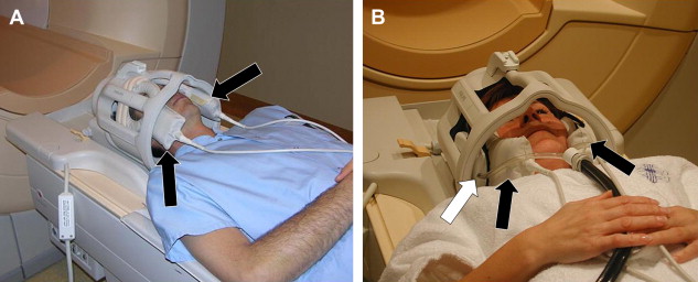
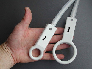
A phased array (synergy) head coil can be used for all cranial nerves. The advantage of a head coil is that it can cover all 12 cranial nerves and that it provides images with good signal-to-noise ratio (S/N) even on the midline and especially in the deepest regions: the cavernous sinus and pre-pontine cistern. A head coil also allows excellent evaluation of the brainstem (cranial nerve nuclei) and brain (eg, olfactory cortex, auditory cortex). Some very small nerves or branches can only be seen when very high resolution is available. This high resolution in combination with enough S/N is especially at 1.5 Tesla often only achievable when synergy surface coils are used. As mentioned above, these coils will only improve the results when one is imaging the more peripherally located nerves (I, II, VII, VIII). These coils can be put inside the head coil, the “concentric coil technique,” so that the head coil can still be used to visualize the deeper structures and complete brain ( Fig. 1 ). At 3 Tesla, the higher S/N often allows production of better images with higher resolution without the need of these surface coils. This also allows the use of different sequences and on 1.5 Tesla, two-dimensional (2D) sequences are still frequently used, at 3 Tesla today nearly all sequences are three-dimensional (3D) sequences and cover all cranial nerves. Finally, microscopic coils can be used ( Fig. 2 ) when very small superficial nerve branches must be visualized. These coils can produce images with extremely high resolution; however, this is only possible when the MR unit is equipped with very strong gradients.
Sequences
The choice of the sequence will depend on the tissue or fluid that is surrounding the nerve.
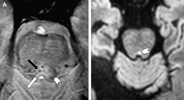
In the brain stem, the cranial nerve nuclei and fascicular segment (nerve segment inside the brain stem) of the nerve cannot be visualized but their location can be deduced when the surrounding myelinated structures are recognized. These are best seen on T2-weighted (T2W), proton-density and especially multi-echo fast field echo (m-FFE) ( Fig. 3 ) or T2∗W 2D spoiled gradient echo multiecho sequence (MEDIC) images. In case of pathology the Flair sequences seem to be the most sensitive and a diffusion sequence is needed to exclude acute infarctions.
Heavily T2W sequences are used once the cisternal segment of the nerve, the segment that is surrounded by cerebrospinal fluid (CSF), is examined. The sequences that are available or used depend highly on the type of MR unit. Typically CISS, 3D-TSE, b-FFE, DRIVE, 3D-FSE, FIESTA, 3D FSE XETA, and so forth sequences are used. All these sequences are heavily T2W 3D-sequences and provide images with very high resolution. However, these sequences should be carefully chosen. Some of these sequences are based on “steady state” (eg, CISS, b-FFF) and produce artifacts at the periphery of the image, especially when a higher spatial resolution is used. Hence, these sequences should be reserved for imaging around the brainstem, in the center of the image. These sequences are better replaced by other type of sequences (3D-TSE, DRIVE) for high resolution imaging of more superficially located nerves (eg, nerves I, VII, VIII) ( Fig. 4 ).
Once the nerves are surrounded by a venous plexus (III to VI in the cavernous sinus, VI behind the clivus in the basilar plexus, IX to XI in the jugular foramen, XII in the hypoglossal canal) they are best seen on high resolution contrast-enhanced Time-Of-Flight MRA images or high resolution 2D (SE or TSE) or 3D (TSE or FFE) T1W images. On these images, the cranial nerves are seen as black structures surrounded by high signal intensity gadolinium-filled venous structures ( Fig. 5 ).
The peripheral segments and branches of the cranial nerves are surrounded by soft tissues and especially fat in the neck and face. High-resolution T1W SE and TSE sequences are in this region best suited to visualize the nerves. The use of fat saturation will make the fat disappear and makes visualization of normal nerves difficult or impossible. Fat saturation has additional value only when an abnormal enhancement of the nerve is expected or must be excluded.
Slice Thickness, In-Plane Resolution
The T2W and proton density SE images through the brainstem have a thickness of 4 mm, to avoid partial volume effect. The in-plane resolution of these images is 0.9 × 0.9 mm.
Coronal 2D T1 SE images can be thicker as there is no risk for partial volume problems as the nerves run antero-posterior and will be visualized anyway. Therefore, for this sequence, all energy is put in in-plane resolution, 0.58 × 0.64 mm while the slice thickness is 4 mm.
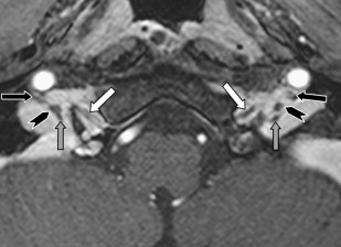
Selective contrast-enhanced T1-weighted FFE images through the cerebellopontine angle (CPA) and jugular foramen (JF) have a slice thickness of 0.625 mm and an in-plane resolution of 0.71 × 0.71 mm. This very thin slice thickness is needed to distinguish the different nerves.
The heavily T2W b-FFE (imaging around brainstem) and DRIVE (imaging more peripherally) have the highest resolution. The b-FFE images are 0.5 mm thick and have an in-plane resolution of 0.5 × 0.5. At 3 Tesla they have a 0.4 3 or even 0.35 3 mm isotropic voxel size. The DRIVE images are 0.35 mm thick and have an in-plane resolution of 0.33 × 0.30, but the 3D slab has only 48 partitions (covers a distance of 17 mm in cranio-caudal direction) while the b-FFE has a somewhat lower spatial resolution but covers a total cranio-caudal distance of up to 12 cm.
Special Techniques/Software
The nerves can be visualized only when the spatial resolution is very high or the voxel size is very small. The time needed to acquire such images is very long with the use of routine sequences. Therefore, any MR technique that speeds up the sequence, without or with minimal loss of S/N, can be used to shorten the examination time and to reduce movement/swallowing/breathing artifacts or can be invested to get even higher resolution in the same time.
Parallel imaging (eg, SENSE) is therefore used in most of the above-mentioned sequences and also helps to reduce susceptibility artifacts in sequences sensitive to this type of artifact (eg, DRIVE, b-FFE). However the maximal SENSE factor that can be used is equal to the number of coil elements used in the phased array coil (if there are only two coil elements, like for the flex S surface coils used for temporal bone imaging, then the acquisition time can maximal be reduced to ½ (1/N° coil elements) with a S/N reduction of the square root of 2 (N° coil elements). This maximal SENSE factor is already causing too much S/N loss when very high resolution imaging of the CPA nerves is performed and that is why routinely a parallel imaging factor of 1.7 is preferred. SENSE is avoided for midline imaging, even when the head coil is used, as the resulting signal drop will immediately degrade the contrast resolution quality of these very high resolution images and consequently make it more difficult to visualize the nerves.
The use of an asymmetric k-space, only possible when TSE types of sequences are used, can reduce the examination time easily by 30%, without the penalty of S/N loss. Hence, this is an ideal technique to increase resolution in the same imaging time or to stick to the same resolution in a shorter examination time.
Cranial nerve anatomy
The Olfactory Nerve or Cranial Nerve I
Olfactory epithelium
The olfactory epithelium is located in the upper one fifth of the nasal cavity and covers the septal and lateral surface of this cavity, including the upper part of the superior turbinate ( Fig. 6 ).
Transethmoidal segment
Bipolar olfactory neurons connect the olfactory epithelium with the olfactory bulbs. These neurons experience a continuous cycle of growth, degeneration, and replacement, which make them “unique” neurons. The dendrites of these olfactory neurons reach the surface of the olfactory epithelium while the unmyelinated axons, about 3 million on each side, run upwards through the openings of the cribriform plate. These axons are grouped in bundles, called filia, which are invested by Schwann cells. This explains why olfactory schwannomas can develop. These filia enter the olfactory bulb and these filia together constitute the real “olfactory nerve.” Some of these filia between the cribriform plate and olfactory bulb can sometimes be seen on high-resolution T2W images ( Fig. 7 ).
Olfactory bulb and tract—intracranial
The olfactory bulb and tract (intracranial) are extensions of the brain and are not a real cranial nerve. The olfactory nerve fibers are received in about 50,000 mitral cells inside the olfactory bulbs. The olfactory bulbs have a convex ovoid shape and can easily be recognized on coronal T2W or T1W images (see Figs. 4, 6, and 7 ). The axons of the olfactory bulb mitral cells are located centrally in the olfactory tract and run from their paramedian origin in the olfactory bulbs posterolaterally toward the anterior border of the anterior perforated substance. Along this course, the olfactory tract follows the inferior border of the olfactory sulcus, located between the gyrus rectus and medial orbital gyrus. The olfactory tract is flatter and more difficult to visualize but its constant position under the olfactory sulcus helps to track this structure ( Fig. 8 ). The olfactory tract divides in lateral, medial, and intermediate stria in front of the anterior perforated substance. This division can be depicted on (para)-axial high-resolution T2W images ( Fig. 8 B).
Olfactory pathways—intracranial
Damage to the olfactory pathway on one side will cause ipsilateral anosmia. Olfaction, and taste are actually the only uncrossed sensations. Some axons in the medial stria reach the septal area via the diagonal band, others cross the midline via the anterior commissure to reach the contralateral olfactory tract. The lateral stria terminates in the piriform lobe (uncus, anterior part of the parahippocampal gyrus, cortical part of the amygdala) and connects through the thalamus (mediodorsal nucleus) with the orbital frontal cortex, which is the highest center for olfactory discrimination. The intermediate stria reach the intermediate cortical olfactory area, a small zone of gray matter at the level of the anterior perforated substance.
The Optic Nerve or Cranial Nerve II
The optic nerve is just like the olfactory bulb and tract; not a true cranial nerve but rather an extension of the brain. The optic nerve can be divided in several segments: intraocular, intraorbital, intracanalicular, and intracranial. The optic pathway then continues in the optic chiasm and optic tracts. The optic radiation and visual cortex are beyond the scope of this chapter.
Intraocular segment
The axons of the retinal ganglion cells form the intraocular optic nerve. This intraocular segment as well as the retina, where the ganglion cells are located, is difficult to visualize. Some of this anatomy can, however, be visualized when microscopic coils and very high resolution are used ( Fig. 9 ). These axons get myelinated by oligodendrocytes as they leave the optic disc.
Intraorbital segment
The intraorbital segment runs through the intraconal space of the orbit, from the globe to the orbital apex and is at that level already surrounded by meninges, explaining the development of many intraorbital meningiomas. The subarachnoid CSF space, located between the pia mater and arachnoid/dura, is surrounding the intraorbital optic nerve and this CSF space is actually in continuity with the CSF of the suprasellar cistern. The nerve and surrounding CSF are best seen on heavily T2W or STIR images. This segment should be imaged with minimal water-fat chemical shift as the nerve-CSF-fat interfaces are otherwise artifacted and difficult to delineate ( Fig. 10 ). The central retinal artery, a branch of the ophthalmic artery, enters the optic nerve with its accompanying vein only in the distal part of the intraorbital segment over a nerve length of 1 cm in the area just behind the globe.
Intracanalicular segment
This segment of the optic nerve inside the optic canal is best seen on MR images ( Fig. 11 ); the bone fragments that can damage the nerve at this site caused by a trauma are of course better seen on CT. Inside this canal the nerve is positioned above the ophthalmic artery.
Intracranial segment
The intracranial segment bridges the gap between the optic canal anterolaterally and optic chiasm posteromedially over a distance of about 10 mm. This nerve segment is covered only by pia mater.
Optic chiasm
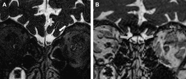
At the optic chiasm, fibers from the temporal hemiretina remain uncrossed and continue in the ipsilateral optic tract. Fibers from the nasal hemiretina cross and continue in the contralateral optic tract. This explains the X-shaped morphology of the chiasm, located just anterior to the pituitary stalk, which is best appreciated on reformatted 3D-T1W images (eg, 3D-FFE, 3D-MPRAGE) or 3D-T2W images (eg, DRIVE, b-FFE) ( Fig. 12 ).
Optic tracts
The continuation of the chiasm in the left and right optic tract can also be visualized. These tracts divide in a smaller medial (containing only 10% of the fibers) and larger lateral root of the optic tract terminating in the medial geniculate body (see Fig. 12 ). These tracts are best distinguished on high-resolution T2W or FLAIR images.
The Oculomotor Nerve or Cranial Nerve III
The oculomotor nerve has a motor function (innervation of five of the extraocular muscles) and a parasympathetic function (innervation of the ciliaris and sphincter pupillae).
Oculomotor nuclear complex
The oculomotor nuclear complex is composed of five individual motor nuclei supplying the extraocular muscles and a more dorsal parasympathetic nucleus of Edinger-Westphal and is located at the level of the superior colliculus. The complex lies between the aqueduct and the red nucleus and is partially embedded in the periaqueductal gray. The structures are best visualized on multi-echo FFE (m-FFE) images ( Fig. 13 ) and the location of the nuclear complex can be deduced from it. The fascicular segment of the oculomotor nerve has an anterolateral course through the midbrain and crosses the medial longitudinal fasciculus (MLF), red nucleus, substantia nigra, and the medial part of the cerebral peduncle.
Cisternal segment
The cisternal segment starts once the nerve leaves the brainstem and enters the interpeduncular cistern. This segment is best seen on high-resolution heavily T2W images ( Fig. 14 ); however, this nerve segment is also large enough to be depicted on T1W images. The nerve passes under the posterior cerebral and above the superior cerebellar artery, continues anteriorly below the posterior communicating artery, and pierces the dural roof of the cavernous sinus.
Cavernous segment
This segment of the third nerve runs in the lateral wall of the cavernous sinus, superolateral to the cavernous internal carotid artery. This segment can best be seen in detail on coronal gadolinium-enhanced high-resolution T1W images through the cavernous sinus but nerve visualization on contrast-enhanced heavily T2W images has also be reported. The third nerve is the nerve with the highest position in the wall of the cavernous sinus. However, just before entering the superior orbital fissure (SOF), the trochlear nerve ascends along the lateral wall of the third nerve and eventually even lies superolateral to the third nerve as they enter the SOF ( Fig. 15 ).
Extracranial segment
The third cranial nerve divides in a superior and inferior branch within the SOF and enters the orbit through this SOF and the annulus of Zinn. The superior branch innervates the superior rectus muscles and levator palpebrae superioris muscles, while the inferior branch innervates the inferior rectus, medial rectus, and inferior oblique muscles. These branches can again be depicted on high-resolution coronal T1W images ( Fig. 16 ). Preganglionic parasympathetic fibers follow the cranial nerve III into the orbit and then exit the branch to the inferior oblique muscle to synapse in the ciliary ganglion. Postganglionic parasympathetic fibers continue as short ciliary nerves and enter the globe by piercing the lamina cribrosa of the sclera. They reach the ciliary body and iris, controlling the papillary sphincter and ciliary muscle.
The Trochlear Nerve or Cranial Nerve IV
The fourth cranial nerve provides motor innervation to only a single muscle, the superior oblique muscle.
Trochlear nucleus
The trochlear nucleus is situated at the level of the inferior colliculus, just ventral to the aqueduct, posterior to the MLF and just inferior to the oculomotor nerve complex. The localization of the nucleus very close to the MLF explains why lesions that involve the trochlear nucleus most often cause both a fourth nerve palsy and an internuclear ophthalmoplegia (INO). Axons leaving the nucleus course dorsally around the aqueduct and the left and right fascicular segments cross each other at the level of the superior medullary velum before exiting the midbrain at its posterior surface, just caudal to the inferior colliculus ( Fig. 17 ). These are two unique features of the fourth cranial nerve: (1) it is the only cranial nerve crossing the midline, hence a superior oblique muscle is always innervated by the contralateral trochlear nucleus and (2) it is the only cranial nerve exiting the brainstem at its dorsal surface.
Cisternal segment
Once outside the brainstem, the nerve is best visualized on heavily T2W images in the axial plane. The nerve is extremely small and is therefore sometimes difficult to find. The trick is to look for the superior medullary velum, a small flat band at the back of the superior part of the fourth ventricle. At that level, the nerves exit the brainstem in a nearly horizontal mediolateral direction until they reach the free edge of the tentorium ( Fig. 18 ). They then course anteriorly around the brainstem and pass through the gap between the superior cerebral artery and superior cerebellar artery, lateral to the oculomotor nerve. Because the nerves have to turn around the complete brainstem, they are the cranial nerves with the longest intracranial segment.
Cavernous segment
The trochlear nerve then enters the lateral wall of the cavernous sinus below the oculomotor nerve ( Fig. 19 ). As already mentioned, the cavernous segment of the trochlear nerve initially is situated below the third nerve but then gradually ascends along the lateral border of the third nerve as the nerves approach the SOF and once in the SOF the trochlear nerve can be found at the superolateral border of the third nerve.
Extracranial segment
The trochlear nerve then crosses over the superior border of the third nerve to run medially toward the superior oblique muscle. This nerve courses above the annulus of Zinn and does not pass through the annulus like the oculomotor and abducens nerve. The cavernous and extracranial segments are again best seen on coronal high resolution T1W images.
The Trigeminal Nerve or Cranial Nerve V
The trigeminal nerve is both motor and sensory to the muscles of mastication and of course also has a large sensory territory.
Trigeminal nuclei—intra-axial segment
Four nuclei, 1 motor and 3 sensory, are located in the brainstem ( Fig. 20 ). The “motor nucleus” is located in the lateral pontine tegmentum and supplies the muscles of mastication and the tensor veli palatini and tensor tympani muscle. The “pontine” or “principal” sensory nucleus (PSN), which can be found lateral to the motor nucleus and anterolateral to the fourth ventricle at the level of the root entry zone (REZ), processes discriminative tactile sensation from the skin of the face. The “mesencephalic nucleus” is a superior extension of the PSN in the midbrain up to the level of the inferior colliculus. It is the only nucleus in the CNS composed of unipolar neurons. It receives afferent fibers for facial proprioception (teeth, hard palate, temporomandibular joint [TMJ]). Their peripheral processes supply stretch receptors in the muscles of mastication and periodontal ligaments of the teeth. The spinal nucleus is a caudal extension of the PSN and descends from the level of the lower pons down to spinal cord level C3. The nucleus merges with dorsal gray matter of the cord. This nucleus mainly receives tactile, nociceptive, and thermal information from the entire V1, V2, and V3 trigeminal areas.