Produce a compensation matrix (.ctm) using the compensation controls containing single stained cells according to the manufacturer’s description or by using the compensation wizard of the IDEAS software. A typical compensation matrix is shown in Fig. 1b.

Apply the compensation matrix (.ctm) to the .rif file of one sample to create a .cif and the corresponding .daf file. The resulting .daf file will be used to generate the template data analysis file (.ast), in which the data analysis tools and gating strategy will be saved. The latter will be used in a batch analysis to create data analysis files (.daf) for each sample.

Use afore created compensated image file (.cif) and the data analysis file (.daf) to define the following gating strategy. Eventually this strategy is saved in an .ast file.

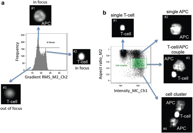
Cells that are not in focus need to be excluded from further evaluations. The gradient RMS feature represents the sharpness quality of the images. Thus, plot the gradient RMS feature within the default mask of the Hoechst33342 staining (M2) and fluorescence channel of the Hoechst33342 staining (Ch2) (encoded as “Gradient RMS_M2_Ch2”) on the x-axis of a histogram (Fig. 2a). Note that Raji B-cells (Fig. 2a, image #1)—that serve as APCs—are bigger than primary human T-cells (Fig. 2a, image #2) and show smaller Gradient “RMS_M2_Ch2” values. Cells out of focus (Fig. 2a, image #3) have “Gradient RMS_M2_Ch2” values smaller than 15. Thus, set a gate that includes all events with “Gradient RMS_M2_Ch2” values bigger than 15.

Create a dot plot which includes cells in focus with the feature “Aspect ratio_M2” (linear scale) on the y-axis. This feature is calculated according to the nuclei stain (Hoechst33342) and a measure of the shape of cells and cell clusters. The feature “Intensity_MC_Ch1”, which corresponds to the side scatter (SSC) is plotted on the x-axis (log scale). This dot plot allows distinguishing T-cell/APC couples (Fig. 2b, image #3) from single T-cells (Fig. 2b, image #1), single APCs (Raji B-cells) (Fig. 2b, image #2), and cell clusters containing 3 or more cells (Fig. 2b, image #4). Define a gate that contains cell couples and control gate borders by clicking on different spots (see Note 4).

Define a T-cell mask according to the upper 60 % of the fluorescence signal of the CD3 staining (“Threshold(M05, Ch5, 60)”, called T-cell-mask) and another mask that determines the immune synapse (called synapse mask, Fig. 3, turquoise areas in images). The latter is a combination of the minimum intensity between the nuclei stains of the T-cell and the APC (Valley-mask) and the aforedefined T-cell mask (“Valley(M02, Ch02, 3) And Threshold(M05, Ch05, 60)”). Calculate the new feature “Area” of both new masks and create a dot plot containing these features (linear scales). This allows gating on T-cell/APC couples with correctly calculated synapse mask (Fig. 3, image #1) and excluding cell couples in which no synapse mask (Fig. 3, image #2) or too big synapse masks. Miscalculated synapse masks occur if the T-cells optically overlap with their APCs (Fig. 3, image #3), if the calculation of the valley-mask was wrong (Fig. 3, image #4) or if two T-cells bind to the same site of the APC (Fig. 3, image #5). The latter will not be excluded by the initial gating on cell couples (compare Fig. 2). The calculations of the area of the T-cell mask enable to exclude T-cell/T-cell couples (Fig. 3, no image shown). Set a gate named “Cell couples corrected” and verify the gating borders by visual evaluation of 10 % of the correct T-cell/APC couples. The error rate should be below 3 %.

Calculate the mean pixel intensity of the fluorescence of the CD3 (Mean Pixel_Synapse_Ch5) and the LFA-1 (Mean Pixel_Synapse_Ch3) staining in the synapse mask (Fig. 4). Calculate a ratio of the mean intensities of the CD3 fluorescence in the synapse and the T-cell mask (Mean Pixel_Synapse_Ch5/Mean Pixel_M5_Ch5) as well as the mean intensities of the fluorescences of LFA-1 in the synapse and the total mean of LFA-1 in T-cells (Mean Pixel_Synapse_Ch3/Mean Pixel_M5_Ch3). These new features are called “CD3 in synapse” and “LFA-1 in synapse” and are plotted in a dot plot (linear scale). Mature immune synapses have values bigger than 1 for both of these features (see Note 5). An oval gate should be defined (border 1–3 for each axis) and then controlled for 10 % of the events. The error rate highly depends on the quality of the staining and should not exceed 5 % enabling to find differences between samples of more that 15 %.