Myocardial Perfusion Imaging with Contrast Echocardiography
Kevin Wei, MD
▪ Introduction
Echocardiography plays an important role in the management of patients, especially in its ability to evaluate left ventricular (LV) global and regional function. Its portability, lack of ionizing radiation, and relatively low cost make it the initial test of choice in many clinical situations. Its clinical utility, however, may be impacted by image quality. It has been estimated that between 10% and 15% of routine echocardiograms, and up to 25% to 30% of studies performed in intensive care units, have incomplete resolution of the endocardial border.1,2 Left ventricular opacification (LVO) with microbubble ultrasound contrast agents (UCAs) have been shown in numerous studies to enhance delineation of the endocardial border, which improves both the qualitative and quantitative assessment of LV function, and decreases inter- and intraobserver variability.3,4,5,6 and 7 LVO has also been shown to improve delineation of intracardiac pathology especially at the LV apex—such as aneurysms and pseudoaneurysms, masses, thrombi, hypertrophic cardiomyopathy, and isolated noncompaction.1 UCAs also enhance delineation of systemic Doppler signals, like pulmonary venous inflows or aortic outflow signals.8
Many may not realize, however, that the imaging methods that are used for LVO today were all developed with an alternate goal in mind—namely, to assess myocardial perfusion with UCAs. Since coronary artery disease (CAD) continues to remain the leading cause of morbidity and mortality worldwide, myocardial perfusion imaging (MPI) with UCAs has wide applications and clinical benefit. However, MPI with UCAs is still an off-label application, because to date, no UCA has yet gained approval from the Federal Drug Administration for an MPI indication.
This chapter will discuss various ultrasound imaging methods that have been developed for qualitative and quantitative assessment of MPI. Furthermore, aspects of the coronary microcirculation that form the basis for MPI with myocardial contrast echocardiography (MCE) will be discussed, as well as the clinical applications that have been studied.
▪ Principles of Quantitative MCE
Properties of Microbubble Tracers
There are currently two commercially available microbubble UCAs in the United States—Optison (GE Healthcare) and Definity (Lantheus Medical Imaging). The mean diameter of the microbubbles is less than 5 µm, allowing them to pass unimpeded through the capillary beds of tissues, and the gas contained within the microbubbles is a high molecular weight gas (perfluoropropane) that has low diffusibility and solubility, so the size of the microbubbles remains stable after their administration into the circulation.
The microbubbles used as tracers during MCE have a number of properties that make them ideal for measuring microcirculatory flow. They approximate the size of red blood cells (RBCs) and can pass unimpeded through the coronary microcirculation.9 The microbubbles are hemodynamically inert and, therefore, do not influence coronary or systemic flow. The microbubbles have also been shown to have the same intravascular rheology as RBCs and can therefore be used to track the transit of RBCs through tissue.10,11
Backscatter signals from microbubbles (see below) are processed into pixels of brightness or acoustic intensity (AI) in the ultrasound system. In order to quantitate the microbubble backscatter signal, the relationship between microbubble concentration and AI must be known. Figure 24-1 shows that at low concentration of microbubbles, the relationship between AI and microbubble concentration is linear (Fig. 24-1, inset).12 As microbubble concentration increases, the AI saturates and the relation between the two variables plateaus. At even higher microbubble concentrations, AI actually decreases due to attenuation of ultrasound by the microbubbles. For quantitative MPI, it is essential to ensure that the microbubble concentration is maintained within the linear range so that the AI remains directly proportional to microbubble concentration. Since it is impractical to derive the microbubble concentration versus AI relation for each patient prior to a perfusion study, a simple way of ensuring that saturation has not been reached within the myocardium is to keep myocardial enhancement visually less bright than the LV cavity.
The Generation and Detection of Microbubble Ultrasound Signal
Ultrasound can be described as a wavefront of alternating positive and negative pressure fluctuations that occur at a frequency above the audible range for humans (>20 KHz). The gas-containing microbubbles are four to five times more compressible than water or tissue. Since microbubbles are compressible and are generally smaller than the wavelength of ultrasound used during clinical
imaging, they undergo volumetric oscillation in the acoustic field since they are compressed during the pressure peaks and expand during the low pressure phases of ultrasound (Fig. 24-2A).13,14 Radial oscillations of microbubbles generate backscatter that result in bright signals in ultrasound images. Myocardial tissue, however, also produces strong ultrasound backscatter. For MPI, in order to detect the microbubbles within the tissue, the system must differentiate microbubble backscatter signals from those of tissue (which is considered “noise” during MCE).
imaging, they undergo volumetric oscillation in the acoustic field since they are compressed during the pressure peaks and expand during the low pressure phases of ultrasound (Fig. 24-2A).13,14 Radial oscillations of microbubbles generate backscatter that result in bright signals in ultrasound images. Myocardial tissue, however, also produces strong ultrasound backscatter. For MPI, in order to detect the microbubbles within the tissue, the system must differentiate microbubble backscatter signals from those of tissue (which is considered “noise” during MCE).
 Figure 24-1. Relation between microbubble concentration and backscatter acoustic intensity. The relation is linear only at low concentrations of microbubbles (inset). (From Skyba DM, Jayaweera AR, Goodman NC, et al. Quantification of myocardial perfusion with myocardial contrast echocardiography during left atrial injection of contrast: implications for venous injection. Circulation 1994;90:1513-1521.) |
An unique property of the oscillating microbubbles is the nonlinear microbubble behavior. Microbubbles have an ideal resonant frequency at which radial oscillation is particularly efficient and exaggerated. The ideal resonant frequency for a microbubble is inversely related to the square of its radius and is also influenced by the viscoelastic and compressive properties of the shell and gas.15,16 By serendipity, for the size and shell properties of currently available microbubble UCAs, the resonant frequency is in the range of those used for echocardiographic imaging in adults. Furthermore, when the acoustic pressure of the insonating beam is sufficiently high, the oscillation of the microbubbles becomes nonlinear, so the alternate compression and expansion of the microbubbles are unequal or asymmetric (Fig. 24-2B).17,18 and 19
The asymmetric acoustic signals from nonlinear microbubble behavior can be shown to consist of fundamental and harmonic frequencies using fast Fourier transform.19 An example of harmonics is illustrated by the frequency-amplitude histogram received from a microbubble contrast agent in Figure 24-2C. A very strong signal is returned at the frequency that was transmitted (the fundamental frequency or fo). A second peak is produced by the microbubbles at twice the fundamental frequency, termed the second harmonic signal (2fo). Tissue produces lower amplitude signals at the second harmonic compared to UCAs and come from gradual distortion of the acoustic pulse as it propagates from the near to the far-field through the tissue.20 Filtering all but the harmonic signals (so-called harmonic imaging) enhances the signal-to-noise ratio during contrast imaging, thereby improving contrast detection compared to fundamental imaging for MPI with MCE.19
The degree of nonlinear oscillation is related to the power of the transmitted ultrasound. Exaggerated microbubble oscillation at high powers leads to microbubble destruction from abrupt fragmentation of the microbubbles, which can occur with only a single pulse of ultrasound. Although intense harmonic backscatter signals can be derived from UCAs as they burst with high-power ultrasound, continual destruction of microbubbles prevents effective contrast enhancement of tissue. Ultrasound systems commonly display the acoustic power in terms of the mechanical index (MI), which is directly proportional to the acoustic pressure (peak negative pressure in MPa) and is inversely proportional to the square root of the frequency. An MI greater than 0.5 usually results in rapid microbubble destruction during imaging. In order to assess myocardial perfusion using high MI imaging methods, the frame rate of imaging must therefore be dramatically reduced to allow microbubbles to populate myocardial capillaries in between destructive pulses. Typically, ultrasound transmission will be triggered using the electrocardiogram, so it was termed “intermittent” imaging. The method initially developed to quantify flow with MCE utilized this type of intermittent high MI imaging (see below).
After intermittent harmonic imaging, the next generation of imaging methods developed to further enhance signal-to-noise ratio for MPI with MCE utilized algorithms that incorporated various receive filters or Doppler processing. As shown in Figure 24-3, amplitude of microbubble backscatter signals (red line at “a”) are of equal intensity to tissue signals (blue line at “b”) at the fundamental frequency (fo), so the signal-to-noise ratio of fundamental imaging is poor and is inadequate for MPI. With second harmonic imaging (transmit at fo with receive only at 2fo), improvement in the signal-to-noise ratio (“c” vs. “d”) is achieved, but strong tissue clutter (“d”) is still present. With the development of broaderband transducers, further improvement in the signal-to-noise ratio (“e” vs. “f”) has been accomplished with ultraharmonic imaging (transmit at fo with receive only at 5/2fo), which takes advantage of low tissue noise (“f”) at the ultraharmonic while microbubble destruction produces strong microbubble signals (“e”). Harmonic and ultraharmonic imaging use B-mode processing techniques to suppress tissue noise, but Doppler processing can also be used. With the latter, received signals from tissue show little spectral decorrelation compared to the transmitted signal, which can then be suppressed by an appropriate wall filter. Conversely, microbubble destruction produces received signals that are markedly different from those transmitted—consequently, only the power spectrum of microbubbles is displayed (this was called power harmonic Doppler imaging).
The use of high MI imaging modes discussed above mandated the use of low frame rates which removed the ability to simultaneously assess myocardial perfusion and wall motion, and also made imaging cumbersome and slow. Therefore, MPI methods using a low MI were sought. When the MI of ultrasound is reduced to very low levels (approximately 0.1), and the frequency of ultrasound approximates the resonant frequency of the microbubble,
nonlinear microbubble oscillation (and harmonic signals) can still be induced without the microbubbles being destroyed. Tissue, on the other hand, responds “linearly” to low MI ultrasound, which means that tissue backscatter contains very low amplitude harmonic signals, making the separation of nonlinear microbubble signals from that of the myocardium possible. Tissue clutter can also be suppressed using multipulse schemes (the transmission of multiple ultrasound pulses sequentially along the same line), where the amplitude (power modulation) or phase (pulse inversion) of sequential pulses are altered. With power modulation (Fig. 24-4), pulses at half-height (“A”) and full-height amplitude (“B”) are transmitted sequentially. The received signals from a linear scatterer such as tissue (Fig. 24-4, Panel A) are identical to the transmitted pulses. Subsequently, the received echoes from the half-height transmitted pulses are scaled and subtracted from the full-height signal, which results in effective removal of tissue clutter. On the other hand, nonlinear scatterers such as microbubbles (Panel B) produce received signals that are different from the transmitted pulses (especially from the full-height pulse), resulting in residual microbubble signal even after subtraction. With pulse
inversion (Fig. 24-5), sequential pulses of inverted phase are transmitted. Again, linear scatterers (Fig. 24-5, Panel A) produce received signals identical to the transmitted pulses, and summation of the received signals results in cancellation of tissue noise. Nonlinear scatterers (Fig. 24-5, Panel B), however, generate signals that cannot be summed. Both power modulation and pulse inversion have also been combined into a single modality (contrast pulse sequencing), where alternate ultrasound pulses have differing amplitude as well as phase.
 Figure 24-2. Panel A: Sound waves cause compressible microbubbles to oscillate, resulting in the production of ultrasound backscatter signals. Panel B: Graph depicting changes in microbubble diameter over time when it is oscillating at its resonant frequency. The alternate expansion and compression phases of the microbubble are unequal (nonlinear). Panel C: The acoustic spectrum arising from nonlinear oscillation of the microbubble contains fundamental and harmonic frequencies. |
 Figure 24-3. Schematic showing backscatter signals derived from microbubbles (red line) and myocardial tissue (blue line) at different frequencies. See text for details. |
The wide array of imaging modalities provides the user with great range and flexibility, and if any particular mode is inadequate for a patient, a different one could be used.
The Coronary Microcirculation
Because the microbubbles used during MCE are pure intravascular tracers, an understanding of the anatomy of the coronary microcirculation is required to appreciate the physiologic information represented by MCE images.
 Figure 24-4. Schematic demonstrating power modulation imaging. Along each line of ultrasound, pulses of different amplitude (A and B) are sequentially transmitted. The backscatter signal derived from the half-height amplitude pulses are summed, and then subtracted from the full-height amplitude pulse. See text for details. |
There is approximately 45 mL of blood in the adult human coronary circulation, which is divided nearly equally between the arterial, venous, and microcirculatory networks.21 Most of the blood in the arterial and venous compartments is located on the epicardial surface of the heart. Within the myocardium itself, microcirculatory myocardial blood volume (MBV) makes up approximately 8% of the LV mass.22 There are approximately 8 million capillaries in the human heart, which contain 90% of the MBV.22 The velocity of blood in the coronary vessels is related to their size. At the capillary level (mean length and diameter of 0.5 mm × 7 µm), the mean red cell velocity at rest is about 1 mm/s. Since the red cells traverse capillaries in single file, it has been estimated that 1 mL of blood would take approximately 1 year to traverse a single capillary!23
When microbubbles are administered as a constant infusion, steady state is achieved after 2 to 3 minutes, where their concentration in any blood pool (LV cavity, myocardium, etc.) is constant and proportional to the blood volume fraction of that pool. Thus, during normal conditions, since MBV represents 8% of LV mass, for every 100 microbubbles within a sample volume in the LV cavity, there will be 8 microbubbles within a similar sized sample volume in the myocardium. The AI measured from the myocardium, when normalized to that from the LV cavity, provides a measure of MBV fraction (since the LV cavity is 100% blood). Because 90% of MBV fraction comprises blood in capillaries, the MCE image provides an assessment of regional myocardial capillary density.
As will be discussed later, the microcirculation not only consists of a channel of passive networks that transports blood through the myocardium, but also an active site of blood flow control as well as metabolic activity. Indeed, the regulation of flow through these networks is complicated and depends on a number of metabolic, myogenic, and other control mechanisms.24 The capillary hydrostatic pressure is continually maintained within the myocardium at approximately 30 mm Hg, with pre- and postcapillary pressures of about 45 and 15 mm Hg, respectively.25 Coronary arterioles (which range in size from 150 to 300 µm) act as a resistance vessels to reduce mean aortic pressure (approximately 90 mm Hg) to the precapillary level.26 These arterioles have smooth muscles with a strong and immediate myogenic response, so arteriolar resistance can change second-to-second in order to keep the precapillary pressure constant (autoregulation).27
 Figure 24-5. Schematic demonstrating pulse inversion imaging. Along each line of ultrasound, sequential pulses of inverted phase are transmitted. The backscatter signals received from tissue and microbubbles are then subtracted from each other. See text for details. |
Quantification of Myocardial Blood Flow with MCE
At steady state, the inflow and outflow of microbubbles in any microcirculatory unit is constant, and is dependent only on the flow rate of microbubbles (which is identical to RBCs) through those vessels. The method for quantification of myocardial blood flow (MBF) with MCE is based on measuring the rate of microbubble transit through the myocardial capillary bed,28 which occurs at a velocity of approximately 1 mm/s at rest, as discussed above.
Microbubbles within the myocardium can be destroyed with high-energy ultrasound, and rapidly eliminated from the myocardium.29 By triggering the transmission of ultrasound to 1 point in the cardiac cycle, new microbubbles are allowed to replenish the microcirculation between destructive pulses of ultrasound, so each image provides a snapshot of the degree of replenishment of the microcirculation in a particular time interval. By making the time interval between destructive pulses longer and longer, more microbubble replenishment can occur and the degree of contrast enhancement increases.
To understand this concept mathematically, assume that all microbubbles within an ultrasound field are destroyed by a single ultrasound pulse and that the elevation (thickness) of the ultrasound beam E is uniform (Fig. 24-6). If new microbubbles enter this field with a flat profile at a velocity v, then the distance (d) they will travel within the beam elevation as the pulsing interval is prolonged (t1 to t4, Fig. 24-6B through E) will be given by the equation E = vt. Thus, as the time interval between consecutive destructive ultrasound pulses is increased, more time is allowed for microbubble replenishment, which is dependent on the velocity of the microbubbles. As pulsing interval lengthens, the rise in microbubble concentration is displayed as a corresponding rise in myocardial AI, provided that the relationship between AI and microbubble concentration remains linear (as discussed above). As shown in Figure 24-6F, when the pulsing interval exceeds T, AI will remain constant. This plateau phase will reflect the effective microbubble concentration within the myocardial microcirculation. At any given concentration of microbubbles, the AI at the plateau phase will be proportional to the sum of the cross-sectional area of microvessels (a) within the beam thickness.
The model predicts a sharp demarcation between the upslope and plateau phases of the pulsing interval-AI relation. In reality, however, neither the beam elevation nor the degree of microbubble destruction are expected to be entirely uniform. The profile of the microbubbles is also not expected to be entirely flat. The actual relationship between AI and pulsing interval is therefore more likely to be curvilinear (Fig. 24-6F) and can be described by the exponential function: y = A(1 — e–βt), where y is AI at a pulsing interval of t, A is the plateau AI, and β is the rate constant that determines the rate of rise of AI.
 Figure 24-6. The elevation dimension (E or thickness) of the ultrasound beam is represented as a rectangle (Panels A to E). At steady state during a continuous infusion of microbubbles, high MI ultrasound is used to destroy all the microbubbles in the elevation (Panel A). As the time interval (t) between successive destructive pulses is prolonged (t1–t4), the degree of microbubble replenishment into the ultrasound elevation increases (d1–d4) and produces greater AI backscatter. The pulsing interval to AI relation (Panel F) can be fitted to an exponential function. See text for details. |
Because the slope of the tangent to the curve is given by dv/dt = AβE–βt, the slope at the origin (t = 0) is Aβ. As shown in Figure 24-6F, this slope is also equal to A/T. Therefore, T = 1/β. Eliminating T between equations results in: v = Eβ. Thus, for a given beam elevation (thickness at a given distance from the transducer), the mean velocity of microbubbles is proportional to β. If flow, f, occurs through an area, a, then: f = av. If E is constant, then a will be proportional to A. Therefore, with rearrangement substitution for v we get: f α AβE. When E is constant, f is proportional to Aβ. If E is known, then v can be expressed in cm/s. Similarly, if the microvascular cross-sectional area is known, then A can be expressed in cm2. The product of A and v will then represent f in mL/s.28
Does it matter whether imaging is performed in diastole or systole during intermittent imaging? After all, it is known that flow in epicardial coronary arteries and veins is phasic in nature. Myocardial vessels fill with blood when myocardial elastance is low in diastole. In systole, the high elastance compresses intramyocardial arterioles which empty out retrogradely.30 Likewise, intramyocardial veins are compressed during systole, which propels blood forward into the coronary sinus.31 Although phasic changes in intramyocardial arteriolar dimensions have been documented during cardiac contraction, what happens to capillary dimensions during this period? We have shown that because arterioles and venules are larger than capillaries, they are compressed in systole prior to capillaries, causing an increase in their resistances that would result in functional isolation of the capillaries (i.e., no flow occurs through the capillaries during systole, but only during diastole).32 Capillary pressure thus increases concurrently with intramyocardial pressure during systole, resulting in fairly constant capillary dimensions throughout the cardiac cycle.32,33 Therefore, for quantification of MBF with MCE using high MI intermittent imaging methods, triggering can be performed at either end-diastole or systole, but the thicker myocardium during systole provides more tissue for evaluation, and the smaller LV cavity produces less far-field attenuation, so triggering during end-systole is recommended.
 Figure 24-7. Contrast-enhanced images from the apical four-chamber view at four different pulsing intervals (Panels A to D). Pulsing interval versus AI plots derived from regions of interest drawn in the septum (orange) and apex (purple) are showing in Panel E. See text for details. |
An excellent linear relationship between absolute MBF measured with radiolabeled microspheres and MCE-derived microbubble velocity has been found in animal studies,28 and significant correlations have been found between positron emission tomographyderived MBF and MCE-derived MBF in humans.34 Thus, MCE allows quantification of MBF velocity (β), MBV (A), and MBF (Aβ) in both experimental and clinical settings.
Figure 24-7 shows an example of how MCE can be used to evaluate regional variations in MBF velocity. In regions where the blood flow velocity is high, there will be greater replenishment of microbubbles into the beam elevation at any given pulsing interval compared to regions with a lower blood flow velocity, resulting in a more rapid rise of AI.28 Panels A to D show images obtained with the pulsing intervals triggered to every 1, 3, 5, and 8 cardiac cycles (corresponding to intervals of approximately 100, 300, 500, and 800 milliseconds at a heart rate of 60 bpm, respectively). Regions of interest have been drawn over the septum and apex to generate theoretical pulsing interval versus AI curves (Panel E) using off-line image analysis software. At the shortest pulsing
interval (Panel A), contrast cannot be seen in any myocardial segment, indicating that the pulsing interval was too short to allow replenishment of measurable amounts of microbubbles into the myocardium. At longer pulsing intervals (Panels B to D), contrast enhancement increases in both beds as more time is available for microbubble replenishment into the microcirculation. The higher flow velocity in the septum results in a greater degree of microbubble replenishment than the apex at any pulsing interval. Thus, the rate of rise of AI from the pulsing interval versus AI curves (Panel E) is higher for the septum (orange line) compared to the apex (purple line).
interval (Panel A), contrast cannot be seen in any myocardial segment, indicating that the pulsing interval was too short to allow replenishment of measurable amounts of microbubbles into the myocardium. At longer pulsing intervals (Panels B to D), contrast enhancement increases in both beds as more time is available for microbubble replenishment into the microcirculation. The higher flow velocity in the septum results in a greater degree of microbubble replenishment than the apex at any pulsing interval. Thus, the rate of rise of AI from the pulsing interval versus AI curves (Panel E) is higher for the septum (orange line) compared to the apex (purple line).
When the pulsing interval is long enough for the entire ultrasound beam elevation to be completely replenished with microbubbles, further increases in pulsing interval do not result in further increases in tissue AI, and the pulsing interval versus AI relation plateaus. As stated earlier, as long as the relation between microbubbles and AI is linear, the steady-state myocardial AI represents myocardial (or capillary) blood volume.24 Since the normal blood flow velocity within the capillaries is very low (approximately 1 mm/s), and the ultrasound beam elevation measures approximately 5 mm in thickness, more than 5 seconds are required between pulses of ultrasound to allow complete replenishment for estimation of capillary blood volume at rest.
The pulsing interval versus myocardial AI relation (Fig. 24-7, Panel E) can be fitted to an exponential function: y = A(1 — e–βt), where y is AI at a PI of t, A is the plateau AI representing MBV, and β represents the mean microbubble velocity. MBF velocity of the septum (βsept) derived from a function fitted to the data points would be found to be greater than βapex.24
Venous Administration of Microbubbles: Bolus or Continuous Infusion
The method described above for assessment of MBF using MCE mandates the use of continuous infusions of microbubbles to achieve “steady-state” concentrations of microbubbles in the circulation. There are other advantages for using continuous infusions. The rate of the infusion can be titrated to attain optimal myocardial opacification and yet avoid significant attenuation. With a bolus injection, high microbubble concentrations at some points during imaging will impede the ability to assess all myocardial segments due to far-field shadowing. Furthermore, excessive concentrations of microbubbles may exceed the linear portion of the relationship between AI and microbubble concentration. Thirdly, a continuous infusion allows time for the acquisition of multiple views, whereas multiple boluses will be required to accomplish the same. A continuous infusion also allows a single operator to perform the entire study alone, without necessitating the presence of a second person to administer the bolus injections.
On the other hand, bolus injections can be performed rapidly. This is especially relevant in the setting of exercise or ionotropic stress, where the time available for image acquisition is limited. With foresight and experience, however, an infusion could be started at an appropriate rate prior to the end of exercise or peak dobutamine stress, so that steady state will already be achieved when it is time to image. A much lower volume of agent is administered with each bolus, so a single vial of the agent is almost always adequate to image every segment even in technically difficult patients where multiple off-axis views are required. A bolus produces higher instantaneous concentrations of microbubbles in the circulation, which is advantageous for low MI techniques that produce smaller backscatter signals from microbubbles.
Overall, our bias is toward the use of continuous infusions because obtaining steady-state concentrations is essential for accurate assessment of the quantitative parameters discussed above, and for reducing attenuation artifacts.
High versus Low Mechanical Index MCE Methods for Quantification of MBF Velocity
More recently, a number of low MI “real-time” MCE techniques have been developed. These techniques produce nonlinear oscillations of microbubbles without destroying them. With low MI imaging, a “flash” impulse consisting of one or several high-power ultrasound frames destroys the microbubbles within the beam elevation, and microbubble replenishment into the microcirculation can then be assessed with continuous imaging at a relatively high frame rate (>15 Hz).35,36 Apart from the ability to visualize both perfusion and myocardial function simultaneously, the main advantage of these techniques for evaluation of MBF is the rapidity with which the entire microbubble replenishment curve can be acquired (15 s compared to >5 min for intermittent imaging techniques).
With real-time imaging, frames throughout the cardiac cycle are acquired after each flash impulse. In contradistinction to intermittent high MI techniques where imaging can be triggered to either systolic or diastolic frames, however, replenishment curves with low MI techniques must be fitted to only end-systolic frames. This is because in diastole, large intramyocardial vessels rapidly replenish with microbubbles due to their high flow velocity (Fig. 24-8, Panel A).37 Fitting a replenishment curve to sequential end-diastolic frames results in overestimation of MBF velocity by 41%.37 Fitting the exponential function to all frames (including diastolic and systolic) within the cardiac cycle will overestimate MBF velocity by 24%.37 The use of end-systolic frames is accurate compared to radiolabeled microspheres (r = 0.53, p = 0.04).37
Since only end-systolic frames should be used for quantification of MBF velocity even with a low MI MCE imaging method, some ultrasound systems allow only end-systolic frames to be digitally acquired while imaging is performed in real time. The sonographer can therefore follow an image on the monitor in real time, but a digital cine-loop of only systolic frames from each cardiac cycle will be acquired, and can subsequently be used for quantification. Most off-line MCE analysis software allows the user to select only the end-systolic frames for use prior to drawing a region of interest. Another method of acquiring only end-systolic frames is achieved by triggering during low MI imaging—so called tissue replenishment imaging. After the flash impulse, low MI imaging is performed at each sequential end-systole over the desired number of cardiac cycles, which are then used to assess microbubble replenishment kinetics.
Despite assessment of only end-systolic frames with both high and low MI imaging techniques, differences in the quantitative parameters are still obtained using the two modalities. The ability of the two modalities to assess the physiologic significance of coronary stenoses have been compared to 99mTc-sestamibi single photon emission computed tomography (SPECT) in patients.38
Intermittent ultraharmonic imaging (high MI) and power modulation Angio (low MI) were performed during continuous infusions of Optison at rest and after dipyridamole stress in 39 patients. 99mTc-sestamibi SPECT was performed simultaneously. MBF velocity and MBF velocity reserve (hyperemic/resting MBF velocity) were quantified from pulsing interval versus AI curves. MBF velocity derived from both MCE methods increased significantly after dipyridamole in normal patients compared to those with either reversible or fixed defects on SPECT. Consequently, MBF velocity reserve was significantly greater in patients with normal perfusion using both techniques. Receiver-operator characteristic curves obtained for MBF velocity reserve provided a sensitivity 82% versus 64% for low MI imaging for detection of defects compared to SPECT. The absolute value of β was also significantly lower during low compared to high MI imaging.
 Figure 24-8. Panel A: Sequential end-diastolic frames acquired after “flash destruction” of microbubbles. In the first end-diastolic frame, linear signals are seen from microbubbles within large intramyocardial arteries. Panel B: Sequential end-systolic frames acquired after “flash destruction of microbubbles.” Panel C: The pulsing interval versus acoustic intensity plots derived from end-diastolic (E-S, orange circles) and end-systolic frames (E-D, green circles). See text for details. |
There are several potential reasons for differences in absolute β between the two types of imaging techniques, as well as for the lower sensitivity of quantitative parameters derived from the low MI technique. Excessive destruction of microbubbles in the LV cavity from multiple flash frames could result in distortion of the myocardial input function and prolongation of the output function. Microbubble destruction may also occur due to high frame rates despite the low MI. Most importantly, however, the variability probably occurs from differences in dynamic range, incorrect curve fitting, and noise between the two techniques.
Nonetheless, due to the relatively ease of image acquisition for real-time low MI techniques compared to high MI-triggered techniques, and the rapidity with which an entire replenishment curve can be derived, the low MI techniques have by-and-large eclipsed the high MI techniques. Although there may be differences in the absolute β between the two types of imaging techniques, regional differences in the rate of replenishment of microbubbles remains valid with low MI techniques.
Stress-Induced Perfusion Defects
So far, this chapter has focused mainly on differences in the rate of replenishment of microbubbles and demonstrated how that parameter can be used to distinguish differences in MBF velocity between perfusion beds. Let us now examine the plateau phase of the pulsing interval versus AI relationship, that is, myocardial or capillary blood volume.
While resting epicardial coronary blood flow remains normal despite the presence of a severe luminal stenosis (up to 85%), flow during maximal hyperemia is reduced when the luminal diameter stenosis severity exceeds 50%.39 It has always been assumed that during maximal hyperemia, the resistance vessels are maximally dilated and the decrease in hyperemic flow is due to resistance offered by the epicardial coronary stenosis. Since they do not have smooth muscle, capillaries have always been thought to be passive conductors of flow.
With MCE, it has been realized that capillary blood volume actually decreases during hyperemia in the presence of a stenosis,
and that this decrease is proportional to stenosis severity.40,41 It is actually the decrease in capillary blood volume that results in perfusion defects on MCE. Since the length of each capillary remains constant, and they cannot dilate or constrict in the absence of smooth muscle, the only way capillary volume can decrease is through the derecruitment of capillary units during hyperemia.
and that this decrease is proportional to stenosis severity.40,41 It is actually the decrease in capillary blood volume that results in perfusion defects on MCE. Since the length of each capillary remains constant, and they cannot dilate or constrict in the absence of smooth muscle, the only way capillary volume can decrease is through the derecruitment of capillary units during hyperemia.
If one examines the distribution of pressures across the coronary circulation, the mean aortic pressure is approximately 90 mm Hg, which is reduced to a precapillary pressure of 45 mm Hg resistance arterioles. There is a further 30 mm Hg drop of pressure across the capillary bed. Each individual capillary is very small and offers high resistance, but since there are so many capillaries in each tissue bed and they are arranged in parallel, the total capillary resistance is relatively small. The drop across the venous bed is only 15 mm Hg since these are high-capacitance vessels, but nevertheless they have some smooth muscle. Thus, at rest, approximately 60% of total myocardial vascular resistance is offered by the arterioles, 25% by the capillaries, and 15% by the venules.41
When hyperemia is induced in the normal coronary circulation, smooth muscle vasodilation results in dilatation of the arterioles and venules with no change in the size of capillaries. The total myocardial vascular resistance can decreases by 68% during hyperemia compared to at rest, with arterial and venular resistances decreasing by 86% and 98%, respectively. Capillary resistance now accounts for 75% of the total myocardial vascular resistance. Thus, capillaries offer the most resistance to MBF during hyperemia and limit the maximal increase in hyperemic MBF.41 Because they are laid in parallel, a greater number of capillaries allows a higher hyperemic MBF and vice versa. Conditions that are associated with capillary loss, such as myocardial infarction, are associated with reduced MBF reserve even in the absence of an epicardial coronary stenosis.
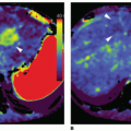
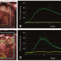
 Figure 24-9. Offline background-subtracted color-coded short-axis images from an experimental study during hyperemia. The images were obtained at baseline (Panel A), and in the presence of a mild (Panel B) or moderate (Panel C) left anterior descending (LAD) coronary artery stenosis. The corresponding pulsing interval versus acoustic intensity curves from the LAD bed (white arrows) are shown (Panel D). See text for details. |
In the presence of a noncritical stenosis during hyperemia, capillary resistance increases due to capillary derecruitment. This likely occurs in an effort to prevent changes in capillary hydrostatic pressure.
It has been shown that the decrease in capillary blood volume distal to a stenosis during hyperemia is proportional to stenosis severity.40,42,43 Therefore, more severe stenoses will be associated with “darker” perfusion defects. Figure 24-9 shows backgroundsubtracted, color-coded short-axis images from an experimental study. All images were obtained during hyperemia, at baseline (Panel A), in the presence of a mild stenosis (trans-stenotic pressure gradient of 14 mm Hg; Panel B), and a moderate stenosis (transstenotic pressure gradient of 22 mm Hg; Panel C) of the left anterior descending coronary artery. The degree of capillary derecruitment, and thus the severity of the perfusion defect becomes greater with increasing levels of stenosis. The corresponding time-intensity curves from the normal and stenosed beds also shows progressive decreases in the peak AI obtained from the stenosed bed with greater stenoses. The ratio of myocardial AI between the stenosed and normal beds during hyperemia was shown to correlate very well with microsphere-derived MBF ratios between the two beds (r = 0.81, p < 0.001).40
Related posts:
 Vascular Anatomy and Microanatomy
 CT and MR Contrast-Enhanced Tissue Perfusion Imaging: Basic Methodology, Postprocessing, Reliability Testing
 Clinical Applications of ASL Brain Perfusion Imaging
 Perfusion CT Imaging in Oncology
 Ultrasound Perfusion Imaging: Techniques and Analytical Methods
 Contrast-Enhanced Ultrasound: Clinical Applications
Stay updated, free articles. Join our Telegram channel

Full access? Get Clinical Tree


