chapter 9 Nuclear Counting Statistics

All measurements are subject to measurement error. This includes physical measurements, such as radiation counting measurements used in nuclear medicine procedures, as well as in biologic and clinical studies, such as evaluation of the effectiveness of an imaging technique. In this chapter, we discuss the type of errors that occur, how they are analyzed, and how, in some cases, they can be minimized.

A Types of Measurement Error

Measurement errors are of three general types: blunders, systematic errors, and random errors.

Blunders are errors that are adequately described by their name. Usually they produce grossly inaccurate results and their occurrence is easily detected. Examples in radiation measurements include the use of incorrect instrument settings, incorrect labeling of sample containers, and injecting the wrong radiopharmaceutical into the patient. When a single value in the data seems to be grossly out of line with others in an experiment, statistical tests are available to determine whether the suspect value may be discarded (see Section E.3). Apart from this there is no way to “analyze” errors of this type, only to avoid them by careful work.

Systematic errors produce results that differ consistently from the correct result by some fixed amount. The same result may be obtained in repeated measurements, but it is the wrong result. For example, length measurements with a warped ruler, or activity measurements with a radiation detector that was miscalibrated or had some other persistent malfunction, could contain systematic errors. Observer bias in the subjective interpretation of data (e.g., scan reading) is another example of systematic error, as is the use for a clinical study of two population groups having underlying differences in some important characteristic, such as different average ages. Measurement results having systematic errors are said to be inaccurate.

It is not always easy to detect the presence of systematic error. Measurement results affected by systematic error may be very repeatable and not too different from the expected results, which may lead to a mistaken sense of confidence. One way to detect systematic error in physical measurements is by the use of measurement standards, which are known from previous measurements with a properly operating system to give a certain measurement result. For example, radionuclide standards, containing a known quantity of radioactivity, are used in various quality assurance procedures to test for systematic error in radiation counting systems. Some of these procedures are described in Chapter 11 , Section D.

Random errors are variations in results from one measurement to the next, arising from physical limitations of the measurement system or from actual random variations of the measured quantity itself. For example, length measurements with an ordinary ruler are subject to random error because of inexact repositioning of the ruler and limitations of the human eye. In clinical or animal studies, random error may arise from differences between individual subjects, for example, in uptake of a radiopharmaceutical. Random error always is present in radiation counting measurements because the quantity that is being measured—namely, the rate of emission from the radiation source—is itself a randomly varying quantity.

Random error affects measurement reproducibility and thus the ability to detect real differences in measured data. Measurements that are very reproducible—in that nearly the same result is obtained in repeated measurements—are said to be precise. It is possible to minimize random error by using careful measurement technique, refined instrumentation, and so forth; however, it is impossible to eliminate it completely. There is always some limit to the precision of a measurement or measurement system. The amount of random error present sometimes is called the uncertainty in the measurement.

It also is possible for a measurement to be precise (small random error) but inaccurate (large systematic error), or vice versa. For example, length measurements with a warped ruler may be very reproducible (precise); nevertheless, they still are inaccurate. On the other hand, radiation counting measurements may be imprecise (because of inevitable variations in radiation emission rates) but still they can be accurate, at least in an average sense.

Because random errors always are present in radiation counting and other measured data, it is necessary to be able to analyze them and to obtain estimates of their magnitude. This is done using methods of statistical analysis. (For this reason, they are also sometimes called statistical errors.) The remainder of this chapter describes these methods of analysis. The discussion focuses on applications involving nuclear radiation-counting measurements; however, some of the methods to be described also are applicable to a wider class of experimental data as discussed in Section E.

B Nuclear Counting Statistics

1 The Poisson Distribution

Suppose that a long-lived radioactive sample is counted repeatedly under supposedly identical conditions with a properly operating counting system. Because the disintegration rate of the radioactive sample undergoes random variations from one moment to the next, the numbers of counts recorded in successive measurements (N₁, N₂, N₃, etc.) are not the same. Given that different results are obtained from one measurement to the next, one might question if a “true value” for the measurement actually exists. One possible solution is to make a large number of measurements and use the average as an estimate for the “true value.”

(9-1)

(9-2)

where n is the number of measurements taken. The notation Σ indicates a sum that is taken over the indicated values of the parameter with the subscript i.

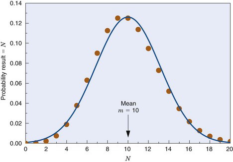
Unfortunately, multiple measurements are impractical in routine practice, and one often must be satisfied with only one measurement. The question then is, how good is the result of a single measurement as an estimate of the true value; that is, what is the uncertainty in this result? The answer to this depends on the frequency distribution of the measurement results. Figure 9-1 shows a typical frequency distribution curve for radiation counting measurements. The solid dots show the different possible results (i.e., number of counts recorded) versus the probability of getting each result. The probability is peaked at a mean value, m, which is the true value for the measurement. Thus if a large number of measurements were made and their results averaged, one would obtain

FIGURE 9-1 Poisson (•) and Gaussian () distributions for mean, m, and variance, σ² = 10.

(9-3)

The solid dots in Figure 9-1 are described mathematically by the Poisson distribution. For this distribution, the probability of getting a certain result N when the true value is m is given by

(9-4)

where e (= 2.718 …) is the base of natural logarithms and N! (N factorial) is the product of all integers up to N (i.e., 1 × 2 × 3 × · · · × N). From Figure 9-1 it is apparent that the probability of getting the exact result N = m is rather small; however, one could hope that the result would at least be “close to” m. Note that the Poisson distribution is defined only for nonnegative integer values of N (0, 1, 2, …).

The probability that a measurement result will be “close to” m depends on the relative width, or dispersion, of the frequency distribution curve. This is related to a parameter called the variance, σ², of the distribution. The variance is a number such that 68.3% (~2/3) of the measurement results fall within ±σ (i.e., square root of the variance) of the true value m. For the Poisson distribution, the variance is given by

(9-5)

Thus one expects to find approximately 2/3 of the counting measurement results within the range of the true value m.

Given only the result of a single measurement, N, one does not know the exact value of m or of σ; however, one can reasonably assume that N ≈ m, and thus that σ ≈ . One can therefore say that if the result of the measurement is N, there is a 68.3% chance that the true value of the measurement is within the range N ± . This is called the “68.3% confidence interval” for m; that is, one is 68.3% confident that m is somewhere within the range N ± .

The range ± is the uncertainty in N. The percentage uncertainty in N is

(9-6)

Example 9-1

Compare the percentage uncertainties in the measurements N₁ = 100 counts and N₂ = 10,000 counts.

Answer

For N₁ = 100 counts, V₁ = 100% / = 10% (Equation 9-6 ). For N₂ = 10,000 counts, V₂ = 100% / = 1%. Thus the percentage uncertainty in 10,000 counts is only 1/10 the percentage uncertainty in 100 counts.

Equation 9-6 and Example 9-1 indicate that large numbers of counts have smaller percentage uncertainties and are statistically more reliable than small numbers of counts.

Other confidence intervals can be defined in terms of σ or . They are summarized in Table 9-1 . The 50% confidence interval (0.675σ) is sometimes called the probable error in N.

TABLE 9-1 CONFIDENCE LEVELS IN RADIATION COUNTING MEASUREMENTS

Range	Confidence Level for m (True Value) (%)
N ± 0.675σ	50
N ± σ	68.3
N ± 1.64σ	90
N ± 2σ	95
N ± 3σ	99.7

2 The Standard Deviation

The variance σ² is related to a statistical index called the standard deviation (SD). The standard deviation is a number that is calculated for a series of measurements. If n counting measurements are made, with results N₁, N₂, N₃, . . ., N_n, and a mean value for those results is found, the standard deviation is

(9-7)

The standard deviation is a measure of the dispersion of measurement results about the mean and is in fact an estimate of σ, the square root of the variance. For radiation counting measurements, one therefore should obtain

(9-8)

This can be used to test whether the random error observed in a series of counting measurements is consistent with that predicted from random variations in source decay rate, or if there are additional random errors present, such as from faulty instrument performance. This is discussed further in Section E.

3 The Gaussian Distribution

When the mean value m is “large,” the Poisson distribution can be approximated by the Gaussian distribution (also called the normal distribution). The equation describing the Gaussian distribution is

(9-9)

where m and σ² are again the mean and variance. Equation 9-9 describes a symmetrical “bell-shaped” curve. As shown by Figure 9-1 , the Gaussian distribution for m = 10 and σ = is very similar to the Poisson distribution for m = 10. For m 20, the distributions are virtually indistinguishable. Two important differences are that the Poisson distribution is defined only for nonnegative integers, whereas the Gaussian distribution is defined for any value of x, and that for the Poisson distribution, the variance σ² is equal to the mean, m, whereas for the Gaussian distribution, it can have any value.

The Gaussian distribution with σ² = m is a useful approximation for radiation counting measurements when the only random error present is that caused by random variations in source decay rate. When additional sources of random error are present (e.g., a random error or uncertainty of ΔN counts caused by variations in sample preparation technique, counting system variations, and so forth), the results are described by the Gaussian distribution with variance given by

(9-10)

The resulting Gaussian distribution curve would be wider than a Poisson curve with σ² = m. The confidence intervals given in Table 9-1 may be used for the Gaussian distribution with this modified value for the variance. For example, the 68.3% confidence interval for a measurement result N would be ± (assuming N ≈ m).

Example 9-2

A 1-mL radioactive sample is pipetted into a test tube for counting. The precision of the pipette is specified as “±2%,” and 5000 counts are recorded from the sample. What is the uncertainty in sample counts per mL?

Answer

The uncertainty in counts arising from pipetting precision is 2% × 5000 counts = 100 counts. Therefore,

and the uncertainty is ≈ 122 counts. Compare this with the uncertainty of ≈ 71 counts that would be obtained without the pipetting uncertainty.

C Propagation of Errors

The preceding section described methods for estimating the random error or uncertainty in a single counting measurement; however, most nuclear medicine procedures involve multiple counting measurements, from which ratios, differences, and so on are used to compute the final result. In the following four sections we describe equations and methods that apply when a result is obtained from a set of counting measurements, N₁, N₂, N₃. . . . In some cases, we present first the general equation applicable for measurements of any type, M₁, M₂, M₃, …, having individual variances, σ (M₁)², σ (M₂)², σ (M₃)², … The general equations can be used to compute the uncertainty in the result for whatever M might represent (e.g., a series of readings from a scale or a thermometer). We then apply these general equations to nuclear counting measurements. Note that in the following subsections it is assumed that random fluctuations in counting measurements arise only from random fluctuations in sample decay rate and that the individual measurements are statistically independent from one another. The latter condition would be violated if N₁ was in some way correlated with N₂, for example, if N₁ was the result for the first half of the counting period for the measurement of N₂.

1 Sums and Differences

For either sums or differences of a series of individual measurements, M₁, M₂, M₃, …, with individual variances, σ (M₁)², σ (M₂)², σ (M₃)², …, the general equation for the variance of the result is given by

(9-11)

Thus, for a series of counting measurements with individual results N₁, N₂, N₃, …

(9-12)

and the percentage uncertainty is

(9-13)

Note that these equations apply to mixed combinations of sums and differences.

2 Constant Multipliers

If a measurement M having variance σ_M² is multiplied by a constant k, the general equation for the variance of the product is

(9-14)

Substituting the appropriate quantities for counting measurements, with M = N

(9-15)

The percentage uncertainty V in the product kN is

(9-16)

which is the same result as Equation 9-6 . Thus there is no statistical advantage gained or lost in multiplying the number of counts recorded by a constant. The percentage uncertainty still depends on the actual number of counts recorded.

3 Products and Ratios

The uncertainty in the product or ratio of a series of measurements M₁, M₂, M₃, … is most conveniently expressed in terms of the percentage uncertainties in the individual results, V₁, V₂, V₃, … The general equation is given by

(9-17)

For counting measurements, this becomes

(9-18)

Again, this expression applies to mixed combinations of products and ratios.

4 More Complicated Combinations

Many nuclear medicine procedures, such as thyroid uptakes and blood volume determinations, use equations of the following general form.

(9-19)

The uncertainty in Y is expressed most conveniently in terms of its percentage uncertainty. Using the rules given previously, one can show that

(9-20)

Example 9-3

A patient is injected with a radionuclide. At some later time a blood sample is withdrawn for counting in a well counter and N_p = 1200 counts are recorded. A blood sample withdrawn prior to injection gives a blood background of N_pb = 400 counts. A standard prepared from the injection preparation records N_s = 2000 counts, and a “blank” sample records an instrument background of N_b = 200 counts. Calculate the ratio of net patient sample counts to net standard counts, and the uncertainty in this ratio.