Patient-specific heart morphology is obtained from short-axis cine magnetic resonance images (MRI). To that end, a robust, data-driven machine learning approach is employed [7] to estimate surface meshes of the left endocardium, left outflow tract, left epicardium, right endocardium, right outflow tract and right inflow tract. Each surface is estimated using marginal space learning and probabilistic boosting trees, constrained by a shape model learned from a database of hundreds of cases, thus ensuring inter-patient point correspondence. Next, each surface is tracked over the entire cine sequence using a combination of tracking by detection and tracking by registration. Finally, the surface meshes at mid-diastole are selected to generate a closed surface of the biventricular myocardium, which is transformed into a tetrahedral volume mesh for simulation¹.

Cardiac electrophysiology (EP) is modelled using the approach presented in [4]. Cardiac transmembrane potentials are calculated according to the mono-domain Mitchell-Schaeffer (MS) model as it offers a good compromise between model observability and fidelity. In this study, we are mostly interested in two parameters: the time during which the ion channels are closed , which captures action potential duration and is directly linked to the QT duration; and tissue diffusivity c, which determines the speed of the electrical wave propagation and is directly linked to the QRS duration. We model fast regional diffusivity for the left and right endocardium to mimic the fast conducting Purkinje network, and slower diffusivity , for the myocardium. Transmembrane potentials are calculated using LBM-EP, a Lattice-Boltzmann method, which is coupled to a boundary element method approach to calculate the 12-lead cardiac electrocardiogram (ECG) resulting from the cardiac potentials [4]. The model is finally personalised like in [8, 9]. BOBYQA, a constrained gradient-free optimization method is used to estimate tissue diffusivity and such that computed QRS duration, QRS electrical axis (EA) and QT duration match the measurements.

The cardiac mechanical model is based on the Bestel-Clement-Sorine (BCS) model [10]. This model describes the heart as a Mooney Rivlin material, and model the stress along the cardiac fibres according to microscopic scale phenomena. Particularly, this model is compatible with the laws of thermodynamics and is able to model the Starling Effect. In this pipeline, it integrates a circulation model representing the 4 phases of the cardiac cycle (aortic pressure modelled by a 4-parameter Windkessel model), and takes the depolarization times and the action potential durations in each point of the mesh as an input to compute the mechanical contraction and relaxation of the myocardium.

As in [3], we only personalize the most influential and independent parameters which are the maximal contraction , the viscosity coefficient , the Bulk Modulus K and the Aortic peripheral resistance Rp. The calibration is performed following [3]: after performing 9 simulations using some specific parameter values that lie in a distribution of acceptable physiological values, the Unscented Transform Algorithm finds in one iteration the set of parameters that best fit the observations within this distribution. In our case, the observations are the minimal LV volume and the time between the two moments the LV is at 50 % of its contraction volume, both calculated from the cine MRI.

One often characterize the variability of a random vector by its mean and covariance matrix since these two first moments completely characterize the Gaussian distribution. However, in more than a few dimensions, the covariance matrix is too large to be computed robustly from only a few data observations. An alternative is to draw just a few samples from the population distribution, either by choosing randomly a number of points from the data observations, or more rationally by selecting a few points that describe the main subspace of variation in the data, for instance through Principal Component Analysis (PCA). Within this subspace one could describe the variability using a minimal number of points thanks to the so-called sigma-points at the vertices of a minimal simplex, originally designed for the Unscented-Kalman Filter [11]. However, it is often empirical observed that using symmetric points on all axes is significantly more accurate for underlying symmetric distributions. This is the approach we took in this study to quantify the variability of the fibre architecture.

We used ex-vivo DTI acquisitions of healthy human hearts, registered in the atlas space [12]. Both left and right ventricles images were generated with this atlas but due to the lower resolution of the right ventricle we chose to use this atlas only for the left ventricle part. On the right ventricle, we instead use a single DTI heart acquisition with high resolution done by Johns Hopkins University (JHU) [13]. Therefore we have no variability estimation of the fibres for the right ventricle.

To compute the mean DTI over the population and quantify the variability, we work in the Log-Euclidean space [14] rather than the standard Euclidean space. The mean DTI is and the data matrix of centred observations is . The PCA is obtained by diagonalizing the large covariance matrix or more efficiently we chose to compute the singular-value decomposition (SVD) of the data matrix , where the diagonal matrix encloses the square root of the eigenvalues of . We choose to only study the first 3 eigenmodes which explain 59 % of the variation of the log-tensors seen in the population. Also we noted that the higher modes being increasingly affected by the noise of the DTI acquisition, they increasingly describe the variability due to the noise and not the intrisic variability. For each mode, we compute two symmetric images representing the range of variation along the mode at plus or minus one standard deviation as: .

In order to relate the atlas space to the geometry of our target patient, we register the mesh of our patient to the mask of both the atlas (for the LV) and the JHU heart (for the RV) with a three-steps framework. First, the mask of the patient is aligned with the mask using a rigid landmark based registration method. Correspondences between the atlas and the target heart are manually checked. Secondly, we perform a similarity registration with five coarse levels and one fine level, each of which are composed of 10 iterations. Finally, we perform a diffeomorphic registration using diffeomorphic demons algorithm with iterations (from coarsest to finest levels), a Gaussian smoothing factor of 2 in the regularization phase, and an interpolation for the moving image done with B-splines  [15]. We then get the full diffeomorphic transformation for each one of our two initial atlases to the target patient mask.

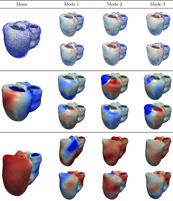
We apply the transformation found in the previous step to the mesh of the patient. For each of the vertices, if the correspondence lies within the RV we use the JHU DTI-image whereas we use the mean or the sampled images of the Lombaert atlas if it lies within the LV. We take the mean (in the Log-Euclidean space) of the tensors of the 5-nearest voxels. The tensor value is then reoriented using the Finite Strain method, and the fibre orientation is taken as its first eigenvector [16]. The results of the fibres personalisation are 7 sets of fibres shown in Fig. 2.

The patient is a 16 years old male who had no family history of cardiac disease. After being admitted at the hospital for chest pain, evidence of reduced ejection fraction and dilated left ventricle led to a first diagnosis of myocarditis. A detailed echocardiographic examination performed 3 month later showed evidence of markedly increased trabeculae of the left ventricular apical and lateral walls, possibly suggesting the presence of left ventricular non-compaction. The MRI study did not confirm this diagnosis but only the idiopathic dilated cardiomyomathy. After 9 month of follow-up in the clinic, the patient was put on the national heart transplant list due to worsening conditions. The patient is now doing well at follow-up after transplant, and the pathology and histology testing at the hospital confirmed the diagnosis of idiopathic dilated cardiomyopathy.