of Myofiber Orientation in High Resolution Phase-Contrast CT Images

and capture the whole volume of the isolated heart (approx. 1 $\times$ 1 $\times$ 2 cm).

2.2 Data Preprocessing

Slicewise segmentation and labeling was performed by visual inspection, discriminating the left and right ventricle and excluding the surrounding container volume, non-tissue artifacts and cavities from the analysis.

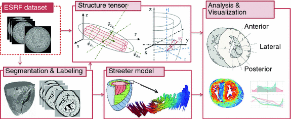
Fig. 1.

Schematic display of the analysis performed on the phase-contrast dataset. The structure tensor box includes a scheme of a fiber system defined with eigenvectors $\mathbf {v_{\lambda }}$ obtained by tensor eigenanalysis, and the assumed cardiac cylindrical coordinate system defined with r-radial, t-tangential and l-longitudinal component. The Streeter model box displays the expected fiber orientation in a whole heart and a transmural patch. The evaluation box shows the sectors selected for quantification of results.

2.3 Gradient Structure Tensor

For calculating the myofiber orientation, a gradient structure tensor method was applied. For each voxel $\mathbf {x}=[x,y,z]$ in the image $I(\mathbf {x})$ , the oriented gradient magnitudes in x, y and z-directions were obtained using a central difference algorithm, resulting in a gradient vector $\mathbf {g}(\mathbf {x}):=\nabla I(\mathbf {x})= [g_x\mathbf {(x)}, g_y\mathbf {(x)},g_z\mathbf {(x)}]$ . The structure tensor in a voxel is defined as $\mathbf {T(x)}:=\nabla I(\mathbf {x}) \nabla I(\mathbf {x}) ^T$ , however, here information is gathered over a voxel’s cubical neighborhood $N(\mathbf {x})$ as a linear combination of the belonging structure tensors, resulting in an local structure tensor estimation $\mathbf {\hat{T} \mathbf {(x)}} = \sum _{\mathbf {p} \in N(\mathbf {p})} {\mathbf {T(p)}}$ , which is in a matrix notation:

$\begin{aligned} \mathbf {\hat{T}} = \left[ \begin{matrix} \sum {{g_x}^2} &{} \sum {g_x g_y} &{} \sum {g_x g_z} \\ \sum {g_y g_x} &{} \sum {{g_y}^2} &{} \sum {g_y g_z} \\ \sum {g_z g_x} &{} \sum {g_z g_y} &{} \sum {{g_z}^2} \end{matrix} \right] \end{aligned}$

(1)

Eigen-decomposition of the structure tensor (Eq. 2) transforms the given gradient space into a space defined with orthogonal vectors $\mathbf {v}_{i}$ $(i \in 1,2,3)$ , encoding the appearance of a tubular structure, i.e. fiber (Fig. 1):

$\begin{aligned} \mathbf {\hat{T}} \mathbf {v} = \mathbf {\lambda } \mathbf {v} \end{aligned}$

(2)

The smallest eigenvalue $\lambda _i$ corresponds to the vector $\mathbf {v}_{i}$ pointing in the fiber direction, while the largest eigenvalue, as opposed to MRI, is assumed to correspond to the vector pointing in the direction of the sheet normal [6]. For the smallest eigenvalue vector, the inclination angle $\alpha _F$ was calculated as an angle between the transverse plane and the vector projection to the local tangential plane of the cylindrical coordinate system of the heart, as illustrated in Fig. 1. In further text, we refer to this angle as fiber angle. Similarly, the transverse angle $\alpha _T$ was calculated as the angle between the tangential plane and the vector projection to the transverse plane. These two angles for each voxel location $\mathbf {x}$ determine the local fiber vector orientation.

The application of the structure tensor method to the fetal cardiac dataset resulted in a fiber vector field and corresponding angle maps.

2.4 Rule-Based Fiber Model

The histological studies [1] performed on cardiac fiber arrangement resulted in a translation of measurements into a mathematical formulation that can be applied to different cardiac geometries [17]. Thus, according to most detailed description for a whole heart available we generated the following Streeter model for the left ventricle (LV) extracted from our data for comparison with the structure tensor method. For each point $\mathbf {x}$ in the LV tissue, two distances are relevant: the smallest distance to the endocardium ( $d_{endo}(\mathbf {x})$ ) and to the epicardium ( $d_{epi}(\mathbf {x})$ ). From these two, a normalized distance map is constructed as:

$\begin{aligned} e(\mathbf {x}) = \frac{d_{endo}(\mathbf {x})}{d_{endo}(\mathbf {x}) + d_{epi}(\mathbf {x})} \end{aligned}$

(3)

representing the normalized tissue thickness. The distance from the point to the base can be expressed with the polar angle $\varPhi (\mathbf {x})$ , with respect to the long axis, defined based on the mitral valve center $\mathbf {x}_{mc}$ and apex $\mathbf {x}_{ap}$ coordinates:

$\begin{aligned} \varPhi (\mathbf {x}) = \arccos \left( \frac{ {(\mathbf {x}_{ap}-\mathbf {x}_{mc})} \cdot (\mathbf {x}-\mathbf {x}_{mc})}{||{\mathbf {x}_{ap}-\mathbf {x}_{mc}}|| \cdot ||\mathbf {x}-\mathbf {x}_{mc}||}\right) \end{aligned}$