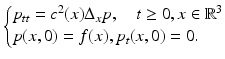
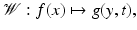
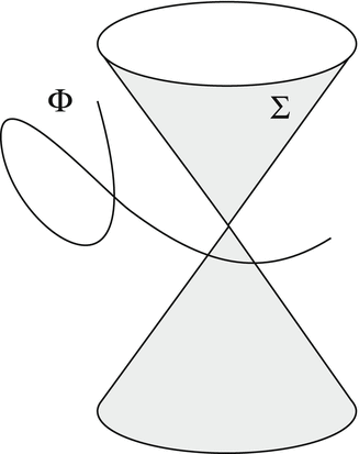
Fig. 1
Thermoacoustic tomography/photoacoustic tomography (TAT/PAT) procedure with a partially surrounding acquisition surface
The physical principle upon which TAT/PAT is based was discovered by Alexander Graham Bell in 1880 [19], and its application for imaging of biological tissues was suggested a century later [21]. It began to be developed as a viable medical imaging technique in the middle of the 1990s [53, 69].
Some of the mathematical foundations of this imaging modality were originally developed starting in the 1990s for the purposes of the approximation theory, integral geometry, and sonar and radar (see [4, 7, 38, 54, 60] for references and extensive reviews of the resulting developments). Physical, biological, and mathematical aspects of TAT/PAT have been recently reviewed in [4, 38, 39, 54, 70, 89, 92, 93, 95].
TAT/PAT is just one, probably the most advanced at the moment, example of the several recently introduced hybrid imaging methods, which combine different types of radiation to yield high quality of imaging unobtainable by single-radiation modalities (see [10, 11, 40, 55, 95] for other examples).
2 Mathematical Models of TAT
In this section, we describe the commonly accepted mathematical model of the TAT procedure and the main mathematical problems that need to be addressed. Since for all our purposes PAT results in the same mathematical model (although the biological features that TAT and PAT detect are different; see details in Ref. [13]), we will refer to TAT only.
Point Detectors and the Wave Equation Model
We will mainly assume that point-like omnidirectional ultrasound transducers, located throughout an observation (acquisition) surface S, are used to detect the values of the pressure p(y, t), where y ∈ S is a detector location and t ≥ 0 is the time of the observation. We also denote by c(x) the speed of sound at a location x. Then, it has been argued that the following model describes correctly the propagating pressure wave p(x, t) generated during the TAT procedure (e.g., [13, 31, 88, 94, 97]):
Here f(x) is the initial value of the acoustic pressure, which one needs to find in order to create the TAT image. In the case of a closed acquisition surface S, we will denote by  the interior domain it bounds. Notice that in TAT the function f(x) is naturally supported inside
  . We will see that this assumption about the support of f sometimes becomes crucial for the feasibility of reconstruction, although some issues can be resolved even if f has nonzero parts outside the acquisition surface.
(1)
the interior domain it bounds. Notice that in TAT the function f(x) is naturally supported inside . We will see that this assumption about the support of f sometimes becomes crucial for the feasibility of reconstruction, although some issues can be resolved even if f has nonzero parts outside the acquisition surface.The data obtained by the point detectors located on a surface S are represented by the function
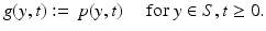
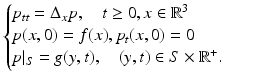
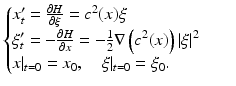
Figure 2 illustrates the space-time geometry of (1).
(2)
Fig. 2
The observation surface S and the domain  containing the object to be imaged
containing the object to be imaged
Thus, the goal in TAT/PAT is to find, using the data g(y, t) measured by transducers, the initial value f(x) at t = 0 of the solution p(x, t) of (3).
We will use the following notation:

Remark 1.
The reader should notice that if a different type of detector is used, the system (1) will still hold, while the measured data will be represented differently from (2) (see section “Variations on the Theme: Planar, Linear, and Circular Integrating Detectors”). This will correspondingly influence the reconstruction procedures.
We can consider the same problem in the space of any dimension, not just in 3D. This is not merely a mathematical abstraction. Indeed, in the case of the so-called integrating line detectors (section “Variations on the Theme: Planar, Linear, and Circular Integrating Detectors”), one deals with the 2D situation.
Acoustically Homogeneous Media and Spherical Means
If the medium being imaged is acoustically homogeneous (i.e., c(x) equals to a constant, which we will assume to be equal to 1 in appropriate units), as it is approximately the case in breast imaging, one deals with the constant coefficient wave equation problem
In this case, the well-known Poisson–Kirchhoff formulas [27, Chap. VI, Sect. 13.2, Formula (15)] for the solution of the wave equation give in 3D
where
is the spherical mean operator applied to the function f(x), dA is the standard area element on the unit sphere in  , and a is a constant. (Versions in all dimensions are known; see (16) and (15).) One can derive from here that knowledge of the function g(x, t) for x ∈ S and all t ≥ 0 is equivalent to knowing the spherical mean Rf(x, t) of the function f for any points x ∈ S and any t ≥ 0. One thus needs to study the spherical mean operator
  , or, more precisely, its restriction to the points x ∈ S only, which we will denote by
  :
:
Due to the connection between the spherical mean operator and the wave equation, one can choose to work with the former, and in fact many works on TAT do so. The spherical mean operator  resembles the classical Radon transform, the common tool of computed tomography [63], which integrates functions over planes rather than spheres. This analogy with Radon transform, although often purely ideological, rather than technical, provides important intuition and frequently points in reasonable directions of study. However, when the medium cannot be assumed to be acoustically homogeneous, and thus c(x) is not constant, the relation between TAT and integral geometric transforms, such as the Radon and spherical mean transforms to a large extent breaks down, and thus one has to work with the wave equation directly.
(5)
(6)
(7)
, and a is a constant. (Versions in all dimensions are known; see (16) and (15).) One can derive from here that knowledge of the function g(x, t) for x ∈ S and all t ≥ 0 is equivalent to knowing the spherical mean Rf(x, t) of the function f for any points x ∈ S and any t ≥ 0. One thus needs to study the spherical mean operator , or, more precisely, its restriction to the points x ∈ S only, which we will denote by :(8)
resembles the classical Radon transform, the common tool of computed tomography [63], which integrates functions over planes rather than spheres. This analogy with Radon transform, although often purely ideological, rather than technical, provides important intuition and frequently points in reasonable directions of study. However, when the medium cannot be assumed to be acoustically homogeneous, and thus c(x) is not constant, the relation between TAT and integral geometric transforms, such as the Radon and spherical mean transforms to a large extent breaks down, and thus one has to work with the wave equation directly.In what follows, we will address both models of TAT (the PDE model and the integral geometry model) and thus will deal with both forward operators  and
and  .
.
and . Main Mathematical Problems Arising in TAT
We now formulate a list of problems related to TAT, which will be addressed in detail in the rest of the article. (This list is more or less standard for a tomographic imaging method.)
Sufficiency of the data:
The first natural question to ask is as follows: Is the data collected on the observation surface S sufficient for the unique reconstruction of the initial pressure f(x) in (3)? In other words, is the kernel of the forward operator  zero? Or, to put it differently, for which sets
  the data collected by transducers placed along S determines f uniquely? Yet another interpretation of this question is through observability of solutions of the wave equation on the set S: does observation on S of a solution of the problem (1) determine the solution uniquely?
zero? Or, to put it differently, for which sets the data collected by transducers placed along S determines f uniquely? Yet another interpretation of this question is through observability of solutions of the wave equation on the set S: does observation on S of a solution of the problem (1) determine the solution uniquely?When the speed of sound is constant, and thus the spherical mean model applies, the equivalent question is whether the operator  has zero kernel on an appropriate class of functions (say, continuous functions with compact support).
has zero kernel on an appropriate class of functions (say, continuous functions with compact support).As it is explained in [7], the choice of precise conditions on the local function class, such as continuity, is of no importance for the answer to the uniqueness question, while behavior at infinity (e.g., compactness of support) is. So, without loss of generality, when discussing uniqueness, one can assume f(x) in (3) to be infinitely differentiable.
Inversion formulas and algorithms:
Since a practitioner needs to see the actual tomogram, rather than just know its existence, the next natural question arises: If uniqueness the data collected on S is established, what are the actual inversion formulas or algorithms? Here again one can work with smooth functions, in the end extending the formulas by continuity to a wider class.
Stability of reconstruction:
If we can invert the transform and reconstruct f from the data g, how stable is the inversion? The measured data are unavoidably corrupted by errors, and stability means that small errors in the data lead to only small errors in the reconstructed tomogram.
Incomplete data problems:
What happens if the data is “incomplete,” for instance, if one can only partially surround the object by transducers? Does this lead to any specific deterioration in the tomogram and if yes, to what kind of deterioration?
Range descriptions:
The next question is known to be important for the analysis of tomographic problems: What is the range of the forward operator  that maps the unknown function f to the measured data g? In other words, what is the space of all possible “ideal” data g(t, y) collected on the surface S? In the constant speed of sound case, this is equivalent to the question of describing the range of the spherical mean operator
  in appropriate function spaces. Such ranges often have infinite co-dimensions, and the importance of knowing the range of Radon type transforms for analyzing problems of tomography is well known. For instance, such information is used to improve inversion algorithms, complete incomplete data, and discover and compensate for certain data errors (e.g., [41, 45, 63, 68, 70] and references therein). In TAT, range descriptions are also closely connected with the speed of sound determination problem listed next (see section “Reconstruction of the Speed of Sound” for a discussion of this connection).
that maps the unknown function f to the measured data g? In other words, what is the space of all possible “ideal” data g(t, y) collected on the surface S? In the constant speed of sound case, this is equivalent to the question of describing the range of the spherical mean operator in appropriate function spaces. Such ranges often have infinite co-dimensions, and the importance of knowing the range of Radon type transforms for analyzing problems of tomography is well known. For instance, such information is used to improve inversion algorithms, complete incomplete data, and discover and compensate for certain data errors (e.g., [41, 45, 63, 68, 70] and references therein). In TAT, range descriptions are also closely connected with the speed of sound determination problem listed next (see section “Reconstruction of the Speed of Sound” for a discussion of this connection).Speed of sound reconstruction:
As the reader can expect, reconstruction procedures require the knowledge of the speed of sound c(x). Thus, the problem arises of the recovery of c(x) either from an additional scan or (preferably) from the same TAT data.
Variations on the Theme: Planar, Linear, and Circular Integrating Detectors
In the most basic and well-studied version of TAT described above, one utilizes point-like broadband transducers to measure the acoustic wave on a surface surrounding the object of interest. The corresponding mathematical model is described by the system (3). In practice, the transducers cannot be made small enough, since smaller detectors yield weaker signals resulting in low signal-to-noise ratios. Smaller transducers are also more difficult to manufacture.
Since finite size of the transducers limits the resolution of the reconstructed images, researchers have been trying to design alternative acquisition schemes using receivers that are very thin but long or wide. Such are 2D planar detectors [24, 43] and 1D linear and circular [23, 42, 73, 103] detectors.
We will assume throughout this section that the speed of sound c(x) is constant and equal to 1.
Planar detectors are made from a thin piezoelectric polymer film glued onto a flat substrate (see, e.g., [75]). Let us assume that the object is contained within the sphere of radius R. If the diameter of the planar detector is sufficiently large (see [75] for details), it can be assumed to be infinite. The mathematical model of such an acquisition technique is no longer described by (3). Let us define the detector plane  by equation x ⋅ ω = s, where ω is the unit normal to the plane and s is the (signed) distance from the origin to the plane. Then, while the propagation of acoustic waves is still modeled by (1), the measured data
  (up to a constant factor which we will, for simplicity, assume to be equal to 1) can be represented by the following integral:
 where dA(x) is the surface measure on the plane. Obviously,
 i.e., the value of g at t = 0 coincides with the integral F(s, ω) of the initial pressure f(x) over the plane
  orthogonal to ω.
by equation x ⋅ ω = s, where ω is the unit normal to the plane and s is the (signed) distance from the origin to the plane. Then, while the propagation of acoustic waves is still modeled by (1), the measured data (up to a constant factor which we will, for simplicity, assume to be equal to 1) can be represented by the following integral: orthogonal to ω.One can show [24, 43] that for a fixed ω, function  is the solution to 1D wave equation
 and thus
![$$\displaystyle\begin{array}{rcl} g_{{\mathrm{planar}}}(s,\omega,t)& =& \frac{1} {2}\left [g_{{\mathrm{planar}}}(s,\omega,s - t) + g_{{\mathrm{planar}}}(s,\omega,s + t)\right ] {}\\ & =& \frac{1} {2}\left [F(s + t,\omega ) + F(s - t,\omega )\right ]. {}\\ \end{array}$$](/wp-content/uploads/2016/04/A183156_2_En_51_Chapter_Equ12.gif) Since the detector can only be placed outside the object, i.e., s ≥ R, the term F(s + t, ω) vanishes, and one obtains
Since the detector can only be placed outside the object, i.e., s ≥ R, the term F(s + t, ω) vanishes, and one obtains
 In other words, by measuring
  , one can obtain values of the planar integrals of f(x). If, as proposed in [24, 43], one conducts measurements for all planes tangent to the upper half sphere of radius R (i.e.,
 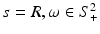 ), then the resulting data yield all values of the standard Radon transform of f(x). Now the reconstruction can be carried out using one of the many known inversion algorithms for the latter transform [63].
is the solution to 1D wave equation, one can obtain values of the planar integrals of f(x). If, as proposed in [24, 43], one conducts measurements for all planes tangent to the upper half sphere of radius R (i.e., ), then the resulting data yield all values of the standard Radon transform of f(x). Now the reconstruction can be carried out using one of the many known inversion algorithms for the latter transform [63].Linear detectors are based on optical detection of acoustic signal. Some of the proposed optical detection schemes utilize as the sensitive element a thin straight optical fiber in combination with Fabry–Perot interferometer [23, 42]. Changes of acoustic pressure on the fiber change (proportionally) its length; this elongation, in turn, is detected by the interferometer. A similar idea is used in [73]; in this work the role of a sensitive element is played by a laser beam passing through the water in which the object of interest is submerged, and thus the measurement does not perturb the acoustic wave. In both cases, the length of the sensitive element exceeds the size of the object, while the diameter of the fiber (or of the laser beam) can be made extremely small (see [75] for a detailed discussion), which removes restrictions on resolution one can achieve in the images.
Let us assume that the fiber (or laser beam) is aligned along the line  , where vectors
  , and ω form an orthonormal basis in
  . Then the measured quantities
 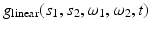 are equal (up to a constant factor which, we will assume, equals to 1) to the following line integral:
 Similar to the case of planar detection, one can show [23, 42, 73] that for fixed vectors
  the measurements
  satisfy the 2D wave equation
 The initial values
  coincide with the line integrals of f(x) along lines
  . Suppose one makes measurements for all values of s 1(τ), s 2(τ) corresponding to a curve
 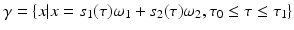 lying in the plane spanned by
  . Then one can try to reconstruct the initial value of g from the values of g on γ. This problem is a 2D version of (3), and thus the known algorithms (see Sect. 4) are applicable.
, where vectors , and ω form an orthonormal basis in . Then the measured quantities are equal (up to a constant factor which, we will assume, equals to 1) to the following line integral: the measurements satisfy the 2D wave equation coincide with the line integrals of f(x) along lines . Suppose one makes measurements for all values of s 1(τ), s 2(τ) corresponding to a curve lying in the plane spanned by . Then one can try to reconstruct the initial value of g from the values of g on γ. This problem is a 2D version of (3), and thus the known algorithms (see Sect. 4) are applicable. In order to complete the reconstruction from data obtained using line detectors, the measurements should be repeated with different directions of ω. For each value of ω, the 2D problem is solved; the solutions of these problems yield values of line integrals of f(x). If this is done for all values of ω lying on a half circle, the set of the recovered line integrals of f(x) is sufficient for reconstructing this function. Such a reconstruction represents the inversion of the well known in tomography X-ray transform. The corresponding theory and algorithms can be found, for instance, in [63].
Finally, the use of circular integrating detectors was considered in [103]. Such a detector can be made out of optical fiber combined with an interferometer. In [103], a closed-form solution of the corresponding inverse problem is found. However, this approach is very new, and neither numerical examples nor reconstructions from real data have been obtained yet.
3 Mathematical Analysis of the Problem
In this section, we will address most of the issues described in section “Main Mathematical Problems Arising in TAT,” except the reconstruction algorithms, which will be discussed in Sect. 4.
Uniqueness of Reconstruction
The problem discussed here is the most basic one for tomography: Given an acquisition surface S along which we distribute detectors, is the data g(y, t) for y ∈ S, t ≥ 0 (see (3)) sufficient for a unique reconstruction of the tomogram f? A simple counting of variables shows that S should be a hypersurface in the ambient space (i.e., a surface in  or a curve in
  ). As we will see below, although there are some simple counterexamples and remaining open problems, for all practical purposes, the uniqueness problem is positively resolved, and most surfaces S do provide uniqueness. We address this issue for acoustically homogeneous media first and then switch to the variable speed case.
or a curve in ). As we will see below, although there are some simple counterexamples and remaining open problems, for all practical purposes, the uniqueness problem is positively resolved, and most surfaces S do provide uniqueness. We address this issue for acoustically homogeneous media first and then switch to the variable speed case.Before doing so, however, we would like to dispel a concern that arises when one looks at the problem of recovering f from g in (3). Namely, an impression might arise that we consider an initial-boundary value (IBV) problem for the wave equation in the cylinder  , and the goal is to recover the initial data f from the known boundary data g. This is clearly impossible, since according to standard PDE theorems (e.g., [27]), one can solve this IBV problem for arbitrary choice of the initial data f and boundary data g (as long as they satisfy simple compatibility conditions, which are fulfilled, for instance, if f vanishes near S and g vanishes for small t, which is the case in TAT). This means that apparently g contains essentially no information about f at all. This argument, however, is flawed, since the wave equation in (3) holds in the whole space, not just in
  . In other words, S is not a boundary, but rather an observation surface. In particular, considering the wave equation in the exterior of S, one can derive that if f is supported inside
  , the boundary values g of the solution p of (3) also determine the normal derivative of p at S for all positive times. Thus, we in fact have (at least theoretically) the full Cauchy data of the solution p on S, which should be sufficient for reconstruction. Another way of addressing this issue is to notice that if the speed of sound is constant, or at least non-trapping (see the definition below in section “Acoustically Inhomogeneous Media”), the energy of the solution in any bounded domain (in particular, in
  ) must decay in time. The decay when
  together with the boundary data g guarantees the uniqueness of solution and thus uniqueness of recovery f.
, and the goal is to recover the initial data f from the known boundary data g. This is clearly impossible, since according to standard PDE theorems (e.g., [27]), one can solve this IBV problem for arbitrary choice of the initial data f and boundary data g (as long as they satisfy simple compatibility conditions, which are fulfilled, for instance, if f vanishes near S and g vanishes for small t, which is the case in TAT). This means that apparently g contains essentially no information about f at all. This argument, however, is flawed, since the wave equation in (3) holds in the whole space, not just in . In other words, S is not a boundary, but rather an observation surface. In particular, considering the wave equation in the exterior of S, one can derive that if f is supported inside , the boundary values g of the solution p of (3) also determine the normal derivative of p at S for all positive times. Thus, we in fact have (at least theoretically) the full Cauchy data of the solution p on S, which should be sufficient for reconstruction. Another way of addressing this issue is to notice that if the speed of sound is constant, or at least non-trapping (see the definition below in section “Acoustically Inhomogeneous Media”), the energy of the solution in any bounded domain (in particular, in ) must decay in time. The decay when together with the boundary data g guarantees the uniqueness of solution and thus uniqueness of recovery f.These arguments, as the reader will see, play a role in understanding reconstruction procedures.
Acoustically Homogeneous Media
We assume here the sound speed c(x) to be constant (in appropriate units, one can choose it to be equal to 1, which we will do to simplify considerations).
In order to state the first important result on uniqueness, let us recall the system (5), allowing an arbitrary dimension n of the space:

(9)
We introduce the following useful definition:
Definition 2.
A set S is said to be a uniqueness set if when used as the acquisition surface, it provides sufficient data for unique reconstruction of the compactly supported tomogram f (i.e., the observed data g in (9) determines uniquely function f). Otherwise, it is called a nonuniqueness set.
In other words, S is a uniqueness set if the forward operator  (or, equivalently,
  ) has zero kernel.
(or, equivalently, ) has zero kernel.We have not indicated above the smoothness class of f(x). However, it is not hard to show (e.g., [7]) that the uniqueness does not depend on the smoothness of f; for simplicity, the reader can assume that f is infinitely differentiable. On the other hand, compactness of support is important in what follows.
We will start with a very general statement about the acquisition (observation) sets S that provide insufficient information for unique reconstruction of f (see [7] for the proof and references):
Theorem 1.
If S is a nonuniqueness set , then there exists a nonzero harmonic polynomial Q, which vanishes on S.
This theorem implies, in particular, that all “bad” (nonuniqueness) observation sets are algebraic, i.e., they have a polynomial vanishing on them. Turning this statement around, we conclude that any set S that is a uniqueness set for harmonic polynomials is sufficient for unique TAT reconstruction (although, as we will see in section “Incomplete Data,” this does not mean practicality of the reconstruction).
The proof of Theorem 1, which the reader can find in [7, 54], is not hard and in fact is enlightening, but providing it would lead us too far from the topic of this survey.
We will consider first the case of closed acquisition surfaces, i.e., the ones that completely surround the object to be imaged. We will address the general situation afterward.
Closed Acquisition Surfaces S
Theorem 2 ([7]).
If the acquisition surface S is the boundary of bounded domain  (i.e., a closed surface), then it is a uniqueness set. Thus, the observed data g in (9) determines uniquely the sought function
  . (The statement holds, even though f is not required to be supported inside S.)
(i.e., a closed surface), then it is a uniqueness set. Thus, the observed data g in (9) determines uniquely the sought function . (The statement holds, even though f is not required to be supported inside S.) Proof.
There is, however, another more intuitive explanation of why Theorem 2 holds true (although it requires somewhat stronger assumptions or a more delicate proof than the one indicated below). Namely, since the solution p of (9) has compactly supported initial data, its energy is decaying inside any bounded domain, in particular inside  (see section “Acoustically Inhomogeneous Media” and [32, 47] and references therein about local energy decay). On the other hand, if there is nonuniqueness, there exists a nonzero f such that g(y, t) = 0 for all y ∈ S and t. This means that we can add homogeneous Dirichlet boundary conditions
  to (9). But then the standard PDE theorems [27] imply that the energy stays constant in
  . Combination of the two conclusions means that p is zero in
  for all times t. It is well known [27] that such a solution of the wave equation must be identically zero everywhere, and thus f = 0.
(see section “Acoustically Inhomogeneous Media” and [32, 47] and references therein about local energy decay). On the other hand, if there is nonuniqueness, there exists a nonzero f such that g(y, t) = 0 for all y ∈ S and t. This means that we can add homogeneous Dirichlet boundary conditions to (9). But then the standard PDE theorems [27] imply that the energy stays constant in . Combination of the two conclusions means that p is zero in for all times t. It is well known [27] that such a solution of the wave equation must be identically zero everywhere, and thus f = 0.This energy decay consideration can be extended to some classes of non-compactly supported functions f of the L p classes, leading to the following result of [1]:
Theorem 3 ([1]).
Let S be the boundary of a bounded domain in  and
and  . Then:

and . Then:1.
If  and the spherical mean of f over almost every sphere centered on S is equal to zero, then f = 0.
and the spherical mean of f over almost every sphere centered on S is equal to zero, then f = 0. 2.
for all f such that  .
.
The previous statement fails when  when
when  and might fail to be such when
 ![$$p > \frac{2n} {n-1}$$” src=”/wp-content/uploads/2016/04/A183156_2_En_51_Chapter_IEq54.gif”></SPAN>.</DIV></DIV><br />
<DIV class=Para>This result shows that the assumption, if not necessarily of compactness of support of <SPAN class=EmphasisTypeItalic>f</SPAN>, but at least of a sufficiently fast decay of <SPAN class=EmphasisTypeItalic>f</SPAN> at infinity, is important for the uniqueness to hold.</DIV></DIV><br />
<DIV id=Sec11 class=]()
when and might fail to be such when General Acquisition Sets S
Theorem 4.
If a set S is not algebraic, or if it contains an open part of a closed analytic surface  , then it is a uniqueness set.
, then it is a uniqueness set. Indeed, the first claim follows immediately from Theorem 1. The second one works out as follows: if an open subset of an analytic surface  is a nonuniqueness set, then by an analytic continuation type argument (see [7]), one can show that the whole
  is such a set. However, this is impossible, due to Theorem 2.
is a nonuniqueness set, then by an analytic continuation type argument (see [7]), one can show that the whole is such a set. However, this is impossible, due to Theorem 2.There are simple examples of nonuniqueness surfaces. Indeed, if S is a plane in 3D (or a line in 2D or a hyperplane in dimension n) and f(x) in (3) is odd with respect to S, then clearly the whole solution of (3) has the same parity and thus vanishes on S for all times t. This means that, if one places transducers on a planar S, they might register zero signals at all times, while the function f to be reconstructed is not zero. Thus, there is no uniqueness of reconstruction when S is a plane. On the other hand (see [27, 51]), if f is supported completely on one side of the plane S (the standard situation in TAT), it is uniquely recoverable from its spherical means centered on S and thus from the observed data g.
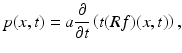
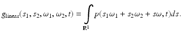
The question arises on what are other “bad” (nonuniqueness) acquisition surfaces than planes. This issue has been resolved in 2D only. Namely, consider a set of N lines on the plane intersecting at a point and forming at this point equal angles. We will call such a figure the Coxeter cross  (see Fig. 3). It is easy to construct a compactly supported function that is odd simultaneously with respect of all lines in
  . Thus, a Coxeter cross is also a nonuniqueness set. The following result, conjectured in [60] and proven in the full generality in [7], shows that up to adding finitely many points, this is all that can happen to nonuniqueness sets:
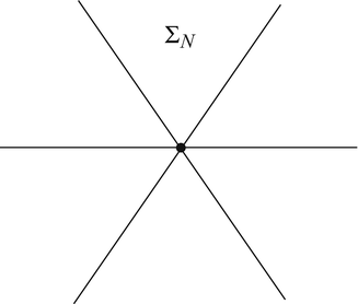
(see Fig. 3). It is easy to construct a compactly supported function that is odd simultaneously with respect of all lines in . Thus, a Coxeter cross is also a nonuniqueness set. The following result, conjectured in [60] and proven in the full generality in [7], shows that up to adding finitely many points, this is all that can happen to nonuniqueness sets:Fig. 3
Coxeter cross of N lines
Theorem 5 ([7]).
A set S in the plane  is a nonuniqueness set for compactly supported functions f, if and only if it belongs to the union
  of a Coxeter cross
  and a finite set of points
  .
.
is a nonuniqueness set for compactly supported functions f, if and only if it belongs to the union of a Coxeter cross and a finite set of points .Again, compactness of support is crucial for the proof provided in [7]. There are no other proofs known at the moment of this result (see the corresponding open problem in Sect. 5). In particular, there is no proven analogue of Theorem 3 for non-closed sets S (unless S is an open part of a closed analytic surface).
The n-dimensional (in particular, 3D) analogue of Theorem 5 has been conjectured [7], but never proven, although some partial advances in this direction have been made in [8, 36].
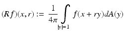
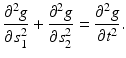
Conjecture 1.
A set S in  is a nonuniqueness set for compactly supported functions f, if and only if it belongs to the union
  , where
  is the cone of zeros of a homogeneous (with respect to some point in
  ) harmonic polynomial, and
  is an algebraic subset of
  of dimension at most n − 2 (see Fig. 4).
is a nonuniqueness set for compactly supported functions f, if and only if it belongs to the union , where is the cone of zeros of a homogeneous (with respect to some point in ) harmonic polynomial, and is an algebraic subset of of dimension at most n − 2 (see Fig. 4).Fig. 4
The conjectured structure of a most general nonuniqueness set in 3D
Uniqueness Results for a Finite Observation Time
So far, we have addressed only the question of uniqueness of reconstruction in the nonpractical case of the infinite observation time. There are, however, results that guarantee the uniqueness of reconstruction for a finite time of observation. The general idea is that it is sufficient to observe for the time that it takes the geometric rays (see section “Acoustically Inhomogeneous Media”) from the interior  of S to reach S. In the case of a constant speed, which we will assume to be equal to 1, the rays are straight and are traversed with the unit speed. This means that if D is the diameter of
  (i.e., the maximal distance between two points in the closure of
  ), then after time t = D, all rays coming from
  have left the domain. Thus, one hopes that waiting till time t = D might be sufficient. In fact, due to the specific initial conditions in (3), namely, that the time derivative of the pressure is equal to zero at the initial moment, each singularity of f emanates two rays, and at least one of them will reach S in time not exceeding D∕2. And indeed, the following result of [36] holds:
of S to reach S. In the case of a constant speed, which we will assume to be equal to 1, the rays are straight and are traversed with the unit speed. This means that if D is the diameter of (i.e., the maximal distance between two points in the closure of ), then after time t = D, all rays coming from have left the domain. Thus, one hopes that waiting till time t = D might be sufficient. In fact, due to the specific initial conditions in (3), namely, that the time derivative of the pressure is equal to zero at the initial moment, each singularity of f emanates two rays, and at least one of them will reach S in time not exceeding D∕2. And indeed, the following result of [36] holds:Theorem 6 ([36]).
If S is smooth and closed surface bounding domain  and D is the diameter of
  , then the TAT data on S collected for the time 0 ≤ t ≤ 0.5D uniquely determines f.
and D is the diameter of , then the TAT data on S collected for the time 0 ≤ t ≤ 0.5D uniquely determines f. Notice that a shorter collection time does not guarantee uniqueness. Indeed, if S is a sphere and the observation time is less than 0. 5D, due to the finite speed of propagation, no information from a neighborhood of the center can reach S during observation. Thus, values of f in this neighborhood cannot be reconstructed.
Acoustically Inhomogeneous Media
We assume that the speed of sound is strictly positive, c(x) > c > 0, and such that c(x) − 1 has compact support, i.e., c(x) = 1 for large x.
Trapping and Non-trapping
We will frequently impose the so-called non-trapping condition on the speed of sound c(x) in  . To introduce it, let us consider the Hamiltonian system in
  with the Hamiltonian
  :
:
The solutions of this system are called bicharacteristics, and their projections into  are rays (or geometric rays).
. To introduce it, let us consider the Hamiltonian system in with the Hamiltonian :(10)
are rays (or geometric rays).Definition 3.
We say that the speed of sound c(x) satisfies the non-trapping condition, if all rays with  tend to infinity when
  .
.
tend to infinity when .The rays that do not tend to infinity are called trapped.
A simple example, where quite a few rays are trapped, is the radial parabolic sound speed c(x) = c | x | 2.
It is well known (e.g., [46]) that singularities of solutions of the wave equation are carried by geometric rays. In order to make this statement more precise, we need to recall the notion of a wave front set WF(u) of a distribution u(x) in  . This set carries detailed information on singularities of u(x).
. This set carries detailed information on singularities of u(x).Definition 4.
Distribution u(x) is said to be microlocally smooth near a point  , where
  , and
, and  , if there is a smooth “cutoff” function ϕ(x) such that ϕ(x 0) ≠ 0 and that the Fourier transform
  of the function ϕ(x)u(x) decays faster than any power
  when
when  , in directions that are close to the direction of
  . (We remind the reader that if this Fourier transform decays that way in all directions, then u(x) is smooth (infinitely differentiable) near the point x 0.)
, where , and , if there is a smooth “cutoff” function ϕ(x) such that ϕ(x 0) ≠ 0 and that the Fourier transform of the function ϕ(x)u(x) decays faster than any power when , in directions that are close to the direction of . (We remind the reader that if this Fourier transform decays that way in all directions, then u(x) is smooth (infinitely differentiable) near the point x 0.)The wave front set  of
of  consists of all pairs
  such that u is not microlocally smooth near
  .
.
of consists of all pairs such that u is not microlocally smooth near .In other words, if  , then u is not smooth near x 0, and the direction of
  indicates why it is not: the Fourier transform does not decay well in this direction. For instance, if u(x) consists of two smooth pieces joined non-smoothly across a smooth interface
  , then WF(u) can only contain pairs
  such that
  and
and  is normal to
  at x.
at x.
, then u is not smooth near x 0, and the direction of indicates why it is not: the Fourier transform does not decay well in this direction. For instance, if u(x) consists of two smooth pieces joined non-smoothly across a smooth interface , then WF(u) can only contain pairs such that and is normal to at x.It is known that the wave front sets of solutions of the wave equation propagate with time along the bicharacteristics introduced above. This is a particular instance of a more general fact that applies to general PDEs and can be found in [46, 84]. As a result, if after time T all the rays leave the domain  of interest, the solution becomes smooth (infinitely differentiable) inside
  .
.
of interest, the solution becomes smooth (infinitely differentiable) inside .The notion of so-called local energy decay, which we survey next, is important for the understanding of the non-trapping conditions in TAT.
Local Energy Decay Estimates
Assuming that the initial data f(x) (1) is compactly supported and the speed c(x) is non-trapping, one can provide the local energy decay estimates [32, 90, 91]. Namely, in any bounded domain  , the solution p(x, t) of (1) satisfies, for a sufficiently large T 0 and for any (k, m), the estimate
 for even n and
  for odd n and some δ > 0. Any value T 0 larger than the diameter of
  works in this estimate.
, the solution p(x, t) of (1) satisfies, for a sufficiently large T 0 and for any (k, m), the estimate for even n and for odd n and some δ > 0. Any value T 0 larger than the diameter of works in this estimate.Uniqueness Result for Non-trapping Speeds
If the speed is non-trapping, the local energy decay allows one to start solving the problem (3) from t = ∞, imposing zero conditions at t = ∞ and using the measured data g as the boundary conditions. This leads to recovery of the whole solution and in particular its initial value f(x). As the result, one obtains the following simple uniqueness result of [3]:
Theorem 7 ([3]).
If the speed c(x) is smooth and non-trapping and the acquisition surface S is closed, then the TAT data g(y,t) determines the tomogram f(x) uniquely.
Notice that the statement of the theorem holds even if the support of f is not completely inside of the acquisition surface S.
Uniqueness Results for Finite Observation Times
As in the case of constant coefficients, if the speed of sound is non-trapping, appropriately long finite observation time suffices for the uniqueness. Let us denote by  the supremum of the time it takes the ray to reach S, over all rays originating in
  . In particular, if c(x) is trapping,
  might be infinite.
the supremum of the time it takes the ray to reach S, over all rays originating in . In particular, if c(x) is trapping, might be infinite.Theorem 8 ([86]).
The data g measured till any time T larger than  is sufficient for the unique recovery of f.
is sufficient for the unique recovery of f. Stability
By stability of reconstruction of the TAT tomogram f from the measured data g, we mean that small variations of g in an appropriate norm lead to small variations of the reconstructed tomogram f, also measured by an appropriate norm. In other words, small errors in the data lead to small errors in the reconstruction.
We will try to give the reader a feeling of the general state of affairs with stability, referring to the literature (e.g., [5, 48, 54, 71, 86]) for further exact details.
We will consider as functional spaces the standard Sobolev spaces H s of smoothness s. We will also denote, as before, by  the operator transforming the unknown f into the data g.
the operator transforming the unknown f into the data g.Let us recall the notions of Lipschitz and Hölder stability . An even weaker logarithmic stability will not be addressed here. The reader can find discussion of the general stability notions and issues, as applied to inverse problems, in [49].
Definition 5.
The operation of reconstructing f from g is said to be Lipschitz stable between the spaces  and
and  , if the following estimate holds for some constant C:
and , if the following estimate holds for some constant C:The reconstruction is said to be Hölder stable (a weaker concept), if there are constants 
.Stability can be also interpreted in the terms of the singular values σ j of the forward operator  in L 2, which have at most power decay when j → ∞. The faster is the decay, the more unstable the reconstruction becomes. The problems with singular values decaying faster than any power of j are considered to be extremely unstable. Even worse are the problems with exponential decay of singular values (analytic continuation or solving Cauchy problem for an elliptic operator belong to this class). Again, the book [49] is a good source for finding detailed discussion of such issues.
in L 2, which have at most power decay when j → ∞. The faster is the decay, the more unstable the reconstruction becomes. The problems with singular values decaying faster than any power of j are considered to be extremely unstable. Even worse are the problems with exponential decay of singular values (analytic continuation or solving Cauchy problem for an elliptic operator belong to this class). Again, the book [49] is a good source for finding detailed discussion of such issues.Consider as an example inversion of the standard in X-ray CT and MRI Radon transform that integrates a function f over hyperplanes in  . It smoothes function by “adding (n − 1)∕2 derivatives.” Namely, it maps continuously H s -functions in
  into the Radon projections of class H s+(n−1)∕2. Moreover, the reconstruction procedure is Lipschitz stable between these spaces (see [63] for detailed discussion).
. It smoothes function by “adding (n − 1)∕2 derivatives.” Namely, it maps continuously H s -functions in into the Radon projections of class H s+(n−1)∕2. Moreover, the reconstruction procedure is Lipschitz stable between these spaces (see [63] for detailed discussion).One should notice that since the forward mapping is smoothing (it “adds derivatives” to a function), the inversion should produce functions that are less smooth than the data, which is an unstable operation. The rule of thumb is that the stronger is the smoothing, the less stable is the inversion (this can be rigorously recast in the language of the decay of singular values). Thus, problems that require reconstructing non-smooth functions from infinitely differentiable (or even worse, analytic) data are extremely unstable (with super-algebraic or exponential decay of singular values correspondingly). This is just a consequence of the standard Sobolev embedding theorems (see, e.g., how this applies in TAT case in [65]).
In the case of a constant sound speed and the acquisition surface completely surrounding the object, as we have mentioned before, the TAT problem can be recast as inversion of the spherical mean transform  (see Sect. 2). Due to analogy between the spheres centered on S and hyperplanes, one can conjecture that the Lipschitz stability of the inversion of the spherical mean operator
  is similar to that of the inversion of the Radon transform. This indeed is the case, as long as f is supported inside S, as has been shown in [71]. In the cases when closed-form inversion formulas are available (see section “Constant Speed of Sound”), this stability can also be extracted from them. If the support of f does reach outside, reconstruction of the part of f that is outside is unstable (i.e., is not even Hölder stable, due to the reasons explained in section “Incomplete Data”).
(see Sect. 2). Due to analogy between the spheres centered on S and hyperplanes, one can conjecture that the Lipschitz stability of the inversion of the spherical mean operator is similar to that of the inversion of the Radon transform. This indeed is the case, as long as f is supported inside S, as has been shown in [71]. In the cases when closed-form inversion formulas are available (see section “Constant Speed of Sound”), this stability can also be extracted from them. If the support of f does reach outside, reconstruction of the part of f that is outside is unstable (i.e., is not even Hölder stable, due to the reasons explained in section “Incomplete Data”).In the case of variable non-trapping speed of sound c(x), integral geometry does not apply anymore, and one needs to address the issue using, for instance, time reversal. In this case, stability follows by solving the wave equation in reverse time starting from t = ∞, as it is done in [3]. In fact, Lipschitz stability in this case holds for any observation time exceeding  (see [86], where microlocal analysis is used to prove this result).
(see [86], where microlocal analysis is used to prove this result).The bottom line is that TAT reconstruction is sufficiently stable, as long as the speed of sound is non-trapping.
However, trapping speed does cause instability [48]. Indeed, since some of the rays are trapped inside  , the information about some singularities never reaches S (no matter for how long one collects the data), and thus, as it is shown in [65], the reconstruction is not even Hölder stable between any Sobolev spaces, and the singular values have super-algebraic decay. See also section “Incomplete Data” below for a related discussion.
, the information about some singularities never reaches S (no matter for how long one collects the data), and thus, as it is shown in [65], the reconstruction is not even Hölder stable between any Sobolev spaces, and the singular values have super-algebraic decay. See also section “Incomplete Data” below for a related discussion. Incomplete Data
In the standard X-ray CT, incompleteness of data arises, for instance, if not all projection angles are accessible or irradiation of certain regions is avoided, or as in the ROI (region of interest) imaging, only the ROI is irradiated.
It is not that clear what incomplete data means in TAT. Usually one says that one deals with incomplete TAT data if the acquisition surface does not surround the object of imaging completely. For instance, in breast imaging it is common that only a half-sphere arrangement of transducers is possible. We will see, however, that incomplete data effects in TAT can also arise due to trapping, even if the acquisition surface completely surrounds the object.
The questions addressed here are the following:
1.
Is the collected incomplete data sufficient for unique reconstruction?
2.
If yes, does the incompleteness of the data have any effect on the stability and quality of the reconstruction?
Uniqueness of Reconstruction
Uniqueness of reconstruction issues can be considered essentially resolved for incomplete data in TAT, at least in most situations of practical interest. We will briefly survey here some of the available results. In what follows, the acquisition surface S is not closed (otherwise the problem is considered to have complete data).
Uniqueness for Acoustically Homogeneous Media
In this case, Theorem 4 contains some useful sufficient conditions on S that guarantee uniqueness. Microlocal results of [7, 61, 85], as well as the PDE approach of [36] further applied in [8], provide also some other conditions. We assemble some of these in the following theorem:
Theorem 9.
Let S be a non-closed acquisition surface in TAT. Each of the following conditions on S is sufficient for the uniqueness of reconstruction of any compactly supported function f from the TAT data collected on S:
Get Clinical Tree app for offline access
1.
Surface S is not algebraic (i.e., there is no nonzero polynomial vanishing on S).
2.
Surface S is a uniqueness set for harmonic polynomials (i.e., there is no nonzero harmonic polynomial vanishing on S).
3.
Surface S contains an open piece of a closed analytic surface  .
.
.4.
Surface S contains an open piece of an analytic surface  separating the space
  such that f is supported on one side of


separating the space such that f is supported on one side of
Related posts:

Stay updated, free articles. Join our Telegram channel
Full access? Get Clinical Tree