Fig. 1.
Primary eigenvectors of the diffusion tensors in the left ventricle (LV) colour-coded by (a) their derived fibre angles showing discontinuities in spatial variation, and (b) fractional anisotropy (FA) showing regions of low FA with corresponding uncertain fibre orientation.
The use of the primary eigenvector alone to derive myocardial fibre angles has two main disadvantages. Firstly, water can diffuse equally in opposite directions, but the primary eigenvector arbitrarily represents just one of these directions. This representation can lead to large discontinuities in fibre angle distributions (see Fig. 1(a)), which can cause problems with FE interpolation of these data. In order to interpolate these spatially discontinuous data within FE models, the eigenvectors are usually phase-unwrapped according to a pre-defined smooth fibre field variation [6], however this method requires prior knowledge of the expected field, and does not eliminate all of the problems with these spatial discontinuities.
The second main issue with eigenanalysis of DTMRI is that in regions of apparent near-isotropic diffusion, the primary eigenvector may not reliably represent the local fibre orientation, as indicated in the inset of Fig. 1(b). Anisotropy in a diffusion process is generally quantified by fractional anisotropy (FA) which ranges from 0 (isotropic diffusion) to 1 (diffusion only along one axis) [20]. Low FA can arise from several factors, including low signal-to-noise ratio in the images [21], or that a single preferred direction does not adequately represent the local tissue microstructure. This can occur, for example, in some regions of myocardial infarct [22], or if there are multiple families of crossing fibres present in the tissue, such as near the inter-ventricular junction of the heart. In the case of crossing fibres, the assumption of a single direction to represent the fibres would need to be re-addressed. On the other hand, if regions of low FA are localised zones of poor image quality, then one could reduce the influence of these data during the fitting of fibre field parameters by incorporating a specialised weighting scheme, such as scaling the fitting error in each voxel by the FA value.
In this study, we present a workflow for parameterising myocardial fibre fields directly from the diffusion tensors without the need to compute eigenvectors or FA values for fibre orientation fitting. This framework not only circumvents issues associated with phase-unwrapping of eigenvectors prior to fibre fitting, but also helps to ensure that the interpolated fibre angles in regions with high FA are better representations of the diffusion tensors in those regions.
2 Methods
2.1 Experimental Data
The experimental study was approved by the Animal Ethics Committee of the University of Auckland and conforms to the National Institutes of Health Guide for the Care and Use of Laboratory Animals (NIH Publication No. 85–23).
The heart from a Wistar-Kyoto (WKY) rat was excised, perfused with St. Thomas’ cardioplegic solution to relax the heart, and then fixed using Bouin’s solution in an approximate end-diastolic state. One week later, DTMRI was performed using a 3D fast spin-echo pulse sequence on a Varian 4.7T MRI scanner. Each image set consisted of 11 or 12 short-axis slices with a thickness of 1.5 mm, and no gap between slices. Each slice contained one non-diffusion weighted anatomical image, and 30 diffusion weighted images. Other imaging parameters were as follows: TE = 15 ms; TR = 3 s; number of averages = 6; field of view (FOV) = 20 mm  20 mm
20 mm  16 mm; in-plane resolution = 128
  64 voxels (zero-pad interpolated to 128
  128 voxels); in-plane voxel dimensions = 156
  m
m  156
156  m.
m.
 20 mm
20 mm  16 mm; in-plane resolution = 128
  64 voxels (zero-pad interpolated to 128
  128 voxels); in-plane voxel dimensions = 156
  m
m  156
156  m.
m.2.2 Fibre Field Parameterisation Workflow
The following workflow (Fig. 2) was developed to parameterise a spatially varying myocardial fibre field directly from the diffusion tensors throughout the LV myocardium.
Step 1: Diffusion tensor calculation. From the non-diffusion weighted signals ( ) and the diffusion weighted signals (
 ) captured in 30 non-collinear directions (i.e.
  ), a diffusion tensor, denoted
  (a symmetric tensor with six independent components), was estimated for each voxel by solving the logarithm of the diffusion equation (Eq. 1) proposed by Basser et al. [10].

where b is the diffusion weighting factor (1462 s/mm for this study). The outer-product
  of the diffusion gradient direction (
 ) was pre-calculated before the system of equations was solved using least-squares to determine the six independent components of
  at each voxel.
 ) and the diffusion weighted signals (
 ) captured in 30 non-collinear directions (i.e.
  ), a diffusion tensor, denoted
  (a symmetric tensor with six independent components), was estimated for each voxel by solving the logarithm of the diffusion equation (Eq. 1) proposed by Basser et al. [10].
(1)
 for this study). The outer-product
  of the diffusion gradient direction (
 ) was pre-calculated before the system of equations was solved using least-squares to determine the six independent components of
  at each voxel.
Step 2: Image segmentation. The analysis was limited to the LV for this study. The entire endocardial and epicardial surfaces of the LV were manually segmented from the non-diffusion images using MATLAB1. During the segmentation, papillary muscles and trabeculae were excluded. Three landmark points (the centroids of the LV base, LV apex, and RV base) were selected to construct an orthogonal cardiac coordinate system with the origin located one-third of the distance from base to apex along the long-axis of the LV, with which the x-axis was aligned. The y-axis was directed from the LV to RV centroids, and the z-axis was directed orthogonal to the x-axis and y-axis from the anterior to posterior of the LV.
Step 3: LV FE geometric model construction. To obtain a model representation of the LV geometry, a prolate ellipsoid-shaped 16-element (4 circumferential, 4-longitudinal and 1-transmural) hexahedral FE model was customised to the surface contours obtained from Step 2. The endocardial and epicardial surfaces of the model were simultaneously fitted using non-linear least squares to best match the corresponding surface data.
Step 4: Field-based parameterisation of LV fibre orientation. In order to parameterise the myofibre orientation field within the LV FE geometric model, we developed a new approach to estimate a smoothly continuous fibre field that best aligned with the diffusion tensors at all voxels within the LV. Firstly, we initialised the FE fibre field by setting the fibre angles ( ) to be
  for the endocardial nodes, and
  for the epicardial nodes. Initial imbrication angles (
 ) of all nodes were set to be
  . These angles were interpolated over the FE model using tricubic Hermite basis functions. Secondly, for each voxel (v), we determined its FE local coordinates within the LV geometric model, and, at that location, we computed the myofibre orientation (
 ) defined by Euler angle rotation (using interpolated
  and
and  ) of vectors initially aligned with the local element axes [23]. Thirdly, a scalar objective function (
 ) was constructed using Eq. 2. At a given voxel, if
  and the direction of maximal diffusion were perfectly aligned, then
  , defined as the dot product of
  with the projection of the diffusion tensor (
 ) in the direction of
  , would be maximal. Conversely,
  would be minimal if
  was aligned with the direction of minimal diffusion. Finally, this objective function was maximised using nonlinear optimisation (least-squares quasi-Newton) by modifying the nodal parameters (
 and
and  ). This procedure was implemented using the open-source Cmgui software package2 [24, 25].
 ) to be
  for the endocardial nodes, and
  for the epicardial nodes. Initial imbrication angles (
 ) of all nodes were set to be
  . These angles were interpolated over the FE model using tricubic Hermite basis functions. Secondly, for each voxel (v), we determined its FE local coordinates within the LV geometric model, and, at that location, we computed the myofibre orientation (
 ) defined by Euler angle rotation (using interpolated
  and
and  ) of vectors initially aligned with the local element axes [23]. Thirdly, a scalar objective function (
 ) was constructed using Eq. 2. At a given voxel, if
  and the direction of maximal diffusion were perfectly aligned, then
  , defined as the dot product of
  with the projection of the diffusion tensor (
 ) in the direction of
  , would be maximal. Conversely,
  would be minimal if
  was aligned with the direction of minimal diffusion. Finally, this objective function was maximised using nonlinear optimisation (least-squares quasi-Newton) by modifying the nodal parameters (
 and
and  ). This procedure was implemented using the open-source Cmgui software package2 [24, 25].


