for a sound speed c(x). This equation can be considered as a model for other hyperbolic equations, and the methods presented here can in some cases be extended to study wave phenomena in other fields such as electromagnetism or elasticity.
We will mostly be interested in inverse problems for the wave equation. In these problems, one has access to certain measurements of waves (the solutions u) on the surface of a medium, and one would like to determine material parameters (the sound speed c) of the interior of the medium from these boundary measurements. A typical field where such problems arise is seismic imaging, where one wishes to determine the interior structure of Earth by making various measurements of waves at the surface. We will not describe seismic imaging applications in more detail here, since they are discussed elsewhere in this volume.
Another feature in this chapter is that we will consistently consider anisotropic materials, where the sound speed depends on the direction of propagation. This means that the scalar sound speed c(x), where  , is replaced by a positive definite symmetric matrix
  , and the wave equation becomes
 Anisotropic materials appear frequently in applications such as in seismic imaging.
, is replaced by a positive definite symmetric matrix , and the wave equation becomesIt will be convenient to interpret the anisotropic sound speed (g jk ) as the inverse of a Riemannian metric, thus modeling the medium as a Riemannian manifold . The benefits of such an approach are twofold. First, the well-established methods of Riemannian geometry become available to study the problems, and second, this provides an efficient way of dealing with the invariance under changes of coordinates present in many anisotropic wave imaging problems. The second point means that in inverse problems in anisotropic media, one can often only expect to recover the matrix (g jk ) up to a change of coordinates given by some diffeomorphism. In practice, this ambiguity could be removed by some a priori knowledge of the medium properties (such as the medium being in fact isotropic, see section “From Boundary Distance Functions to Riemannian Metric”).
2 Background
This chapter contains three parts which discuss different topics related to wave imaging. The first part considers the inverse problem of determining a sound speed in a wave equation from the response operator, also known as the hyperbolic Dirichlet-to-Neumann map, by using the boundary control method; see [5, 7, 42]. The second part considers other types of boundary measurements of waves, namely, the scattering relation and boundary distance function, and discusses corresponding inverse problems. The third part is somewhat different in nature and does not consider any inverse problems but rather gives an introduction to the use of curvelet decompositions in wave imaging for nonsmooth sound speeds. We briefly describe these three topics.
Wave Imaging and Boundary Control Method
Let us consider an isotropic wave equation. Let  be an open, bounded set with smooth boundary
  , and let c(x) be a scalar-valued positive function in
  modeling the wave speed in
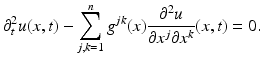
  . First, we consider the wave equation
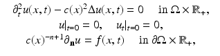
where  denotes the Euclidean normal derivative and n is the unit interior normal. We denote by
  the solution of (1) corresponding to the boundary source term f.
be an open, bounded set with smooth boundary , and let c(x) be a scalar-valued positive function in modeling the wave speed in . First, we consider the wave equation(1)
denotes the Euclidean normal derivative and n is the unit interior normal. We denote by the solution of (1) corresponding to the boundary source term f.Let us assume that the domain  is known. The inverse problem is to reconstruct the wave speed c(x) when we are given the set
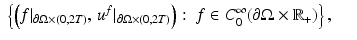 that is, the Cauchy data of solutions corresponding to all possible boundary sources
  , T ∈ (0, ∞]. If T = ∞, then this data is equivalent to the response operator
which is also called the nonstationary Neumann-to-Dirichlet map . Physically,  describes the measurement of the medium response to any applied boundary source f, and it is equivalent to various physical measurements. For instance, measuring how much energy is needed to force the boundary value
  to be equal to any given boundary value
  is equivalent to measuring the map
  on
on  ; see [42, 44]. Measuring
  is also equivalent to measuring the corresponding Neumann-to-Dirichlet map for the heat or the Schrödinger equations or measuring the eigenvalues and the boundary values of the normalized eigenfunctions of the elliptic operator
  ; see [44].
is known. The inverse problem is to reconstruct the wave speed c(x) when we are given the set, T ∈ (0, ∞]. If T = ∞, then this data is equivalent to the response operator(2)
describes the measurement of the medium response to any applied boundary source f, and it is equivalent to various physical measurements. For instance, measuring how much energy is needed to force the boundary value to be equal to any given boundary value is equivalent to measuring the map on ; see [42, 44]. Measuring is also equivalent to measuring the corresponding Neumann-to-Dirichlet map for the heat or the Schrödinger equations or measuring the eigenvalues and the boundary values of the normalized eigenfunctions of the elliptic operator ; see [44].The inverse problems for the wave equation and the equivalent inverse problems for the heat or the Schrödinger equations go back to works of M. Krein at the end of the 1950s, who used the causality principle in dealing with the one-dimensional inverse problem for an inhomogeneous string,  ; see, for example, [46]. In his works, causality was transformed into analyticity of the Fourier transform of the solution. A more straightforward hyperbolic version of the method was suggested by A. Blagovestchenskii at the end of 1960s to 1970s [12, 13]. The multidimensional case was studied by M. Belishev [4] in the late 1980s who understood the role of the PDE control for these problems and developed the boundary control method for hyperbolic inverse problems in domains of Euclidean space. Of crucial importance for the boundary control method was the result of D. Tataru in 1995 [77, 79] concerning a Holmgren-type uniqueness theorem for nonanalytic coefficients. The boundary control method was extended to the anisotropic case by M. Belishev and Y. Kurylev [7]. The geometric version of the boundary control method which we consider in this chapter was developed in [7, 41, 42, 47]. We will consider the inverse problem in the more general setting of an anisotropic wave equation in an unbounded domain or on a non-compact manifold. These problems have been studied in detail in [39, 43] also in the case when the measurements are done only on a part of the boundary. In this paper we present a simplified construction method applicable for non-compact manifolds in the case when measurements are done on the whole boundary. We demonstrate these results in the case when we have an isotropic wave speed c(x) in a bounded domain of Euclidean space. For this, we use the fact that in the Euclidean space, the only conformal deformation of a compact domain fixing the boundary is the identity map. This implies that after the abstract manifold structure (M, g) corresponding to the wave speed c(x) in a given domain
  is constructed, we can construct in an explicit way the embedding of the manifold M to the domain
  and determine c(x) at each point
  . We note on the history of this result that using Tataru’s unique continuation result [77], Theorem 2 concerning this case can be proven directly using the boundary control method developed for domains in Euclidean space in [4].
; see, for example, [46]. In his works, causality was transformed into analyticity of the Fourier transform of the solution. A more straightforward hyperbolic version of the method was suggested by A. Blagovestchenskii at the end of 1960s to 1970s [12, 13]. The multidimensional case was studied by M. Belishev [4] in the late 1980s who understood the role of the PDE control for these problems and developed the boundary control method for hyperbolic inverse problems in domains of Euclidean space. Of crucial importance for the boundary control method was the result of D. Tataru in 1995 [77, 79] concerning a Holmgren-type uniqueness theorem for nonanalytic coefficients. The boundary control method was extended to the anisotropic case by M. Belishev and Y. Kurylev [7]. The geometric version of the boundary control method which we consider in this chapter was developed in [7, 41, 42, 47]. We will consider the inverse problem in the more general setting of an anisotropic wave equation in an unbounded domain or on a non-compact manifold. These problems have been studied in detail in [39, 43] also in the case when the measurements are done only on a part of the boundary. In this paper we present a simplified construction method applicable for non-compact manifolds in the case when measurements are done on the whole boundary. We demonstrate these results in the case when we have an isotropic wave speed c(x) in a bounded domain of Euclidean space. For this, we use the fact that in the Euclidean space, the only conformal deformation of a compact domain fixing the boundary is the identity map. This implies that after the abstract manifold structure (M, g) corresponding to the wave speed c(x) in a given domain is constructed, we can construct in an explicit way the embedding of the manifold M to the domain and determine c(x) at each point . We note on the history of this result that using Tataru’s unique continuation result [77], Theorem 2 concerning this case can be proven directly using the boundary control method developed for domains in Euclidean space in [4].The reconstruction of non-compact manifolds has been considered also in [11, 27] with different kind of data, using iterated time reversal for solutions of the wave equation. We note that the boundary control method can be generalized also for Maxwell and Dirac equations under appropriate geometric conditions [50, 51], and its stability has been analyzed in [1, 45].
Travel Times and Scattering Relation
The problem considered in the previous section of recovering a sound speed from the response operator is highly overdetermined in dimensions n ≥ 2. The Schwartz kernel of the response operator depends on 2n variables, and the sound speed c depends on n variables.
In section “Travel Times and Scattering Relation,” we will show that other types of boundary measurements in wave imaging can be directly obtained from the response operator. One such measurement is the boundary distance function , a function of 2n − 2 variables, which measures the travel times of shortest geodesics between boundary points. The problem of determining a sound speed from the travel times of shortest geodesics is the inverse kinematic problem . The more general problem of determining a Riemannian metric (corresponding to an anisotropic sound speed) up to isometry from the boundary distance function is the boundary rigidity problem . The problem is formally determined if n = 2 but overdetermined for n ≥ 3.
This problem arose in geophysics in an attempt to determine the inner structure of the Earth by measuring the travel times of seismic waves. It goes back to Herglotz [37] and Wiechert and Zoeppritz [84] who considered the case of a radial metric conformal to the Euclidean metric. Although the emphasis has been in the case that the medium is isotropic, the anisotropic case has been of interest in geophysics since the Earth is anisotropic. It has been found that even the inner core of the Earth exhibits anisotropic behavior [24].
To give a proper definition of the boundary distance function, we will consider a bounded domain  with smooth boundary to be equipped with a Riemannian metric g, that is, a family of positive definite symmetric matrices
  depending smoothly on
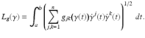
  . The length of a smooth curve
 ![$$\gamma: [a,b] \rightarrow \overline{\Omega }$$](/wp-content/uploads/2016/04/A183156_2_En_52_Chapter_IEq25.gif) is defined to be
is defined to be
 The distance function d g (x, y) for
  is the infimum of the lengths of all piecewise smooth curves in
  joining x and y. The boundary distance function is d g (x, y) for
  .
.
with smooth boundary to be equipped with a Riemannian metric g, that is, a family of positive definite symmetric matrices depending smoothly on . The length of a smooth curve is defined to be is the infimum of the lengths of all piecewise smooth curves in joining x and y. The boundary distance function is d g (x, y) for .In the boundary rigidity problem, one would like to determine a Riemannian metric g from the boundary distance function d g . In fact, since  for any diffeomorphism
  which fixes each boundary point, we are looking to recover from d g the metric g up to such a diffeomorphism. Here,
  is the pullback of g by ψ.
for any diffeomorphism which fixes each boundary point, we are looking to recover from d g the metric g up to such a diffeomorphism. Here, is the pullback of g by ψ.It is easy to give counterexamples showing that this cannot be done in general; consider, for instance, the closed hemisphere, where boundary distances are given by boundary arcs so making the metric larger in the interior does not change d g . Michel [55] conjectured that a simple metric g is uniquely determined, up to an action of a diffeomorphism fixing the boundary, by the boundary distance function d g (x, y) known for all x and y on  . A metric is called simple if for any two points in
  , there is a unique length minimizing geodesic joining them, and if the boundary is strictly convex.
. A metric is called simple if for any two points in , there is a unique length minimizing geodesic joining them, and if the boundary is strictly convex.The conjecture of Michel has been proved for two-dimensional simple manifolds [60]. In higher dimensions, it is open, but several partial results are known, including the recent results of Burago and Ivanov for metrics close to Euclidean [15] and close to hyperbolic [16] (see the survey [40]). Earlier and related works include results for simple metrics conformal to each other [8, 10, 26, 56–58], for flat metrics [34], for locally symmetric spaces of negative curvature [9], for two-dimensional simple metrics with negative curvature [25, 59], a local result [70], a semiglobal solvability result [54], and a result for generic simple metrics [71].
In case the metric is not simple, instead of the boundary distance function, one can consider the more general scattering relation which encodes, for any geodesic starting and ending at the boundary, the start point and direction, the end point and direction, and the length of the geodesic. We will see in section “Travel Times and Scattering Relation” that also this information can be determined directly from the response operator. If the metric is simple, then the scattering relation and boundary distance function are equivalent, and either one is determined by the other.
The lens rigidity problem is to determine a metric up to isometry from the scattering relation. There are counterexamples of manifolds which are trapping, and the conjecture is that on a nontrapping manifold the metric is determined by the scattering relation up to isometry. We refer to [72] and the references therein for known results on this problem.
Curvelets and Wave Equations
In section “Curvelets and Wave Equations,” we describe an alternative approach to the analysis of solutions of wave equations, based on a decomposition of functions into basic elements called curvelets or wave packets . This approach also works for wave speeds of limited smoothness unlike some of the approaches presented earlier. Furthermore, the curvelet decomposition yields efficient representations of functions containing sharp wave fronts along curves or surfaces, thus providing a common framework for representing such data and analyzing wave phenomena and imaging operators. Curvelets and related methods have been proposed as computational tools for wave imaging, and the numerical aspects of the theory are a subject of ongoing research.
A curvelet decomposition was introduced by Smith [67] to construct a solution operator for the wave equation with C 1, 1 sound speed and to prove Strichartz estimates for such equations. This started a body of research on L p estimates for low-regularity wave equations based on curvelet-type methods; see, for instance, Tataru [80–82], Smith [68], and Smith and Sogge [69]. Curvelet decompositions have their roots in harmonic analysis and the theory of Fourier integral operators, where relevant works include Córdoba and Fefferman [23] and Seeger et al. [65] (see also Stein [73]).
In a rather different direction, curvelet decompositions came up in image analysis as an optimally sparse way of representing images with C 2 edges; see Candés and Donoho [20] (the name “curvelet” was introduced in [19]). The property that curvelets yield sparse representations for wave propagators was studied in Candés and Demanet [17, 18]. Numerical aspects of curvelet-type methods in wave computation are discussed in [21, 30]. Finally, both theoretical and practical aspects of curvelet methods related to certain seismic imaging applications are studied in [2, 14, 29, 31, 64].
3 Mathematical Modeling and Analysis
Boundary Control Method
Inverse Problems on Riemannian Manifolds
Let  be an open, bounded set with smooth boundary
  and let c(x) be a scalar-valued positive function in
  , modeling the wave speed in
  . We consider the closure
  as a differentiable manifold M with a smooth, nonempty boundary. We consider also a more general case, and allow (M, g) to be a possibly non-compact, complete manifold with boundary. This means that the manifold contains its boundary
  and M is complete with metric d g defined below. Moreover, near each point x ∈ M, there are coordinates (U, X), where U ⊂ M is a neighborhood of x and
  if x is an interior point, or
  if x is a boundary point such that for any coordinate neighborhoods (U, X) and
  , the transition functions
  are C ∞ -smooth. Note that all compact Riemannian manifolds are complete according to this definition. Usually we denote the components of X by
  .
.
be an open, bounded set with smooth boundary and let c(x) be a scalar-valued positive function in , modeling the wave speed in . We consider the closure as a differentiable manifold M with a smooth, nonempty boundary. We consider also a more general case, and allow (M, g) to be a possibly non-compact, complete manifold with boundary. This means that the manifold contains its boundary and M is complete with metric d g defined below. Moreover, near each point x ∈ M, there are coordinates (U, X), where U ⊂ M is a neighborhood of x and if x is an interior point, or if x is a boundary point such that for any coordinate neighborhoods (U, X) and , the transition functions are C ∞ -smooth. Note that all compact Riemannian manifolds are complete according to this definition. Usually we denote the components of X by .Let u be the solution of the wave equation
Here,  is a real-valued function, and A = A(x, D) is an elliptic partial differential operator of the form

where  is a smooth, symmetric, real, positive definite matrix,
  , and μ(x) > 0 and q(x) are smooth real-valued functions. On existence and properties of the solutions of Eq. (3), see [52]. The inverse of the matrix
  , denoted
  defines a Riemannian metric on M. The tangent space of M at x is denoted by T x M, and it consists of vectors p which in local coordinates (U, X),
  are written as
  . Similarly, the cotangent space T x ∗ M of M at x consists of covectors which are written in the local coordinates as
  . The inner product which g determines in the cotangent space T x ∗ M of M at the point x is denoted by
  for
for  . We use the same notation for the inner product at the tangent space T x M, that is,
  for p, q ∈ T x M.
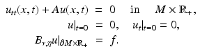
(3)
is a real-valued function, and A = A(x, D) is an elliptic partial differential operator of the form(4)
is a smooth, symmetric, real, positive definite matrix, , and μ(x) > 0 and q(x) are smooth real-valued functions. On existence and properties of the solutions of Eq. (3), see [52]. The inverse of the matrix , denoted defines a Riemannian metric on M. The tangent space of M at x is denoted by T x M, and it consists of vectors p which in local coordinates (U, X), are written as . Similarly, the cotangent space T x ∗ M of M at x consists of covectors which are written in the local coordinates as . The inner product which g determines in the cotangent space T x ∗ M of M at the point x is denoted by for . We use the same notation for the inner product at the tangent space T x M, that is, for p, q ∈ T x M.The metric defines a distance function, which we call also the travel time function,
 where | μ | denotes the length of the path μ, and the infimum is taken over all piecewise C 1-smooth paths μ: [0, 1] → M with μ(0) = x and μ(1) = y.
We define the space L 2(M, dV μ ) with inner product
 where
where  . By the above assumptions, A is formally self-adjoint, that is,

. By the above assumptions, A is formally self-adjoint, that is,Furthermore, let
 where
where  is a smooth function and
 where
where  is the interior conormal vector field of
  , satisfying
  for all cotangent vectors of the boundary,
  . We assume that ν is normalized, so that
  . If M is compact, then the operator A in the domain
  , where H s (M) denotes the Sobolev spaces on M, is an unbounded self-adjoint operator in
  .
.
is a smooth function and is the interior conormal vector field of , satisfying for all cotangent vectors of the boundary, . We assume that ν is normalized, so that . If M is compact, then the operator A in the domain , where H s (M) denotes the Sobolev spaces on M, is an unbounded self-adjoint operator in .An important example is the operator
on a bounded smooth domain  with
with  , where
  is the Euclidean normal derivative of v.
(5)
with , where is the Euclidean normal derivative of v.We denote the solutions of (3) by
 For the initial boundary value problem (3), we define the nonstationary Robin-to-Dirichlet map or the response operator
  by
by
The finite time response operator  corresponding to the finite observation time T > 0 is given by
by(6)
corresponding to the finite observation time T > 0 is given by(7)
For any set  , we denote
  . This means that we identify the functions and their zero continuations.
, we denote . This means that we identify the functions and their zero continuations.By [78], the map  can be extended to bounded linear map
  when
when  is compact. Here,
  denotes the Sobolev space on
  . Below we consider
  also as a linear operator
  , where
  denotes the compactly supported functions in
  .
.
can be extended to bounded linear map when is compact. Here, denotes the Sobolev space on . Below we consider also as a linear operator , where denotes the compactly supported functions in .For t > 0 and a relatively compact open set  , let
, let
This set is called the domain of influence of  at time t.
, let(8)
at time t.When  is an open relatively compact set and
  , it follows from finite speed of wave propagation (see, e.g., [38]) that the wave
  is supported in the domain
  , that is,

is an open relatively compact set and , it follows from finite speed of wave propagation (see, e.g., [38]) that the wave is supported in the domain , that is,(9)
We will consider the boundary of the manifold  with the metric
  inherited from the embedding
  . We assume that we are given the boundary data, that is, the collection
where  is considered as a smooth Riemannian manifold with a known differentiable and metric structure and
  is the nonstationary Robin-to-Dirichlet map given in (6).
with the metric inherited from the embedding . We assume that we are given the boundary data, that is, the collection(10)
is considered as a smooth Riemannian manifold with a known differentiable and metric structure and is the nonstationary Robin-to-Dirichlet map given in (6).Our goal is to reconstruct the isometry type of the Riemannian manifold (M, g), that is, a Riemannian manifold which is isometric to the manifold (M, g). This is often stated by saying that we reconstruct (M, g) up to an isometry. Our next goal is to prove the following result:
Theorem 1.
Let (M,g) to be a smooth, complete Riemannian manifold with a nonempty boundary. Assume that we are given the boundary data (10). Then it is possible to determine the isometry type of manifold (M,g).
From Boundary Distance Functions to Riemannian Metric
In order to reconstruct (M, g), we use a special representation, the boundary distance representation, R(M), of M and later show that the boundary data (10) determine R(M). We consider next the (possibly unbounded) continuous functions  . Let us choose a specific point
  and a constant C 0 > 0 and using these, endow
  with the metric

. Let us choose a specific point and a constant C 0 > 0 and using these, endow with the metric(11)
Consider a map  ,
,
that is,  is the distance function from x ∈ M to the points on
  . The image
  of R is called the boundary distance representation of M. The set R(M) is a metric space with the distance inherited from
  which we denote by d C , too. The map R, due to the triangular inequality, is Lipschitz,
We note that when M is compact and C 0 = diam (M), the metric  is a norm which is equivalent to the standard norm
  of
of  .
.
,(12)
is the distance function from x ∈ M to the points on . The image of R is called the boundary distance representation of M. The set R(M) is a metric space with the distance inherited from which we denote by d C , too. The map R, due to the triangular inequality, is Lipschitz,(13)
is a norm which is equivalent to the standard norm of .We will see below that the map 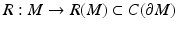 is an embedding. Many results of differential geometry, such as Whitney or Nash embedding theorems, concern the question how an abstract manifold can be embedded to some simple space such as a higher dimensional Euclidean space. In the inverse problem, we need to construct a “copy” of the unknown manifold in some known space, and as we assume that the boundary is given, we do this by embedding the manifold M to the known, although infinite dimensional function space
  .
.
is an embedding. Many results of differential geometry, such as Whitney or Nash embedding theorems, concern the question how an abstract manifold can be embedded to some simple space such as a higher dimensional Euclidean space. In the inverse problem, we need to construct a “copy” of the unknown manifold in some known space, and as we assume that the boundary is given, we do this by embedding the manifold M to the known, although infinite dimensional function space .Next we recall some basic definitions on Riemannian manifolds; see, for example, [22] for an extensive treatment. A path μ: [a, b] → N is called a geodesic if, for any c ∈ [a, b], there is ![$$\varepsilon > 0$$” src=”/wp-content/uploads/2016/04/A183156_2_En_52_Chapter_IEq105.gif”></SPAN> such that if <SPAN class=EmphasisTypeItalic>s</SPAN>, <SPAN class=EmphasisTypeItalic>t</SPAN> ∈ [<SPAN class=EmphasisTypeItalic>a</SPAN>, <SPAN class=EmphasisTypeItalic>b</SPAN>] such that <SPAN id=IEq106 class=InlineEquation><IMG alt=](/wp-content/uploads/2016/04/A183156_2_En_52_Chapter_IEq106.gif) , the path μ([s, t]) is a shortest path between its endpoints, that is,
, the path μ([s, t]) is a shortest path between its endpoints, that is,
![$$\displaystyle{\vert \mu ([s,t])\vert = d_{g}\big(\mu (s),\mu (t)\big).}$$](/wp-content/uploads/2016/04/A183156_2_En_52_Chapter_Equd.gif) In the future, we will denote a geodesic path μ by γ and parameterize γ with its arclength s, so that
In the future, we will denote a geodesic path μ by γ and parameterize γ with its arclength s, so that ![$$\vert \mu ([s_{1},s_{2}])\vert = d_{g}\big(\mu (s_{1}),\mu (s_{2})\big)$$](/wp-content/uploads/2016/04/A183156_2_En_52_Chapter_IEq107.gif) . Let x(s),
. Let x(s),
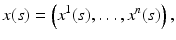 be the representation of the geodesic γ in local coordinates (U, X). In the interior of the manifold, that is, for
  the path x(s) satisfies the second-order differential equations
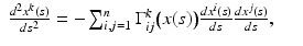
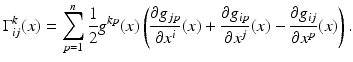
where  are the Christoffel symbols, given in local coordinates by the formula
 Let y ∈ M and
  be a unit vector satisfying the condition
  . Then, we can consider the solution of the initial value problem for the differential equation (14) with the initial data
 This initial value problem has a unique solution x(s) on an interval
  such that
  , or
, or  in case no such s 0 exists. We will denote
  and say that the geodesic is a normal geodesic starting at y if
  and
and  .
.
, the path μ([s, t]) is a shortest path between its endpoints, that is,. Let x(s), the path x(s) satisfies the second-order differential equations(14)
are the Christoffel symbols, given in local coordinates by the formula be a unit vector satisfying the condition . Then, we can consider the solution of the initial value problem for the differential equation (14) with the initial data such that , or in case no such s 0 exists. We will denote and say that the geodesic is a normal geodesic starting at y if and .Example 1.
In the case when (M, g) is such a compact manifold that all geodesics are the shortest curves between their endpoints and all geodesics can be continued to geodesics that hit the boundary, we can see that the metric spaces (M, d g ) and  are isometric. Indeed, for any two points x, y ∈ M, there is a geodesic γ from x to a boundary point z, which is a continuation of the geodesic from x to y. As in the considered case the geodesics are distance minimizing curves, we see that
 and thus
  . Combining this with the triangular inequality, we see that
  for x, y ∈ M and R is isometry of (M, d g ) and
  .
.
are isometric. Indeed, for any two points x, y ∈ M, there is a geodesic γ from x to a boundary point z, which is a continuation of the geodesic from x to y. As in the considered case the geodesics are distance minimizing curves, we see that. Combining this with the triangular inequality, we see that for x, y ∈ M and R is isometry of (M, d g ) and .Notice that when even M is a compact manifold, the metric spaces (M, d g ) and  are not always isometric. As an example, consider a unit sphere in
  with a small circular hole near the South pole of, say, diameter
  . Then, for any x, y on the equator and
  ,
,  and
and  . Then
  , while d g (x, y) may be equal to π.
are not always isometric. As an example, consider a unit sphere in with a small circular hole near the South pole of, say, diameter . Then, for any x, y on the equator and , and . Then , while d g (x, y) may be equal to π.Next, we introduce the boundary normal coordinates on M. For a normal geodesic  starting from
  consider
  . For small s,
and z is the unique nearest point to γ z, ν (s) on  . Let τ(z) ∈ (0, ∞] be the largest value for which (15) is valid for all s ∈ [0, τ(z)]. Then for s > τ(z),
 and z is no more the nearest boundary point for γ z, ν (s). The function
  is called the cut locus distance function, and the set
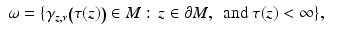
is the cut locus of M with respect to  . The set ω is a closed subset of M having zero measure. In particular, M∖ω is dense in M. In the remaining domain M∖ω, we can use the coordinates
where  is the unique nearest point to x and
  . (Strictly speaking, one also has to use some local coordinates of the boundary,
  and define that

are the boundary normal coordinates.) Using these coordinates, we show that  is an embedding. The result of Lemma 1 is considered in detail for compact manifolds in [42].
starting from consider . For small s,(15)
. Let τ(z) ∈ (0, ∞] be the largest value for which (15) is valid for all s ∈ [0, τ(z)]. Then for s > τ(z), is called the cut locus distance function, and the set(16)
. The set ω is a closed subset of M having zero measure. In particular, M∖ω is dense in M. In the remaining domain M∖ω, we can use the coordinates(17)
is the unique nearest point to x and . (Strictly speaking, one also has to use some local coordinates of the boundary, and define that(18)
is an embedding. The result of Lemma 1 is considered in detail for compact manifolds in [42].Lemma 1.
Let (M,d g ) be the metric space corresponding to a complete Riemannian manifold (M,g) with a nonempty boundary. The map R: (M,d g ) → (R(M),d C ) is a homeomorphism. Moreover, given R(M) as a subset of  , it is possible to construct a distance function d R on R(M) that makes the metric space (R(M),d R ) isometric to (M,d g ).
, it is possible to construct a distance function d R on R(M) that makes the metric space (R(M),d R ) isometric to (M,d g ). Proof.
We start by proving that R is a homeomorphism. Recall the following simple result from topology:
Assume that X and Y are Hausdorff spaces, X is compact, and F: X → Y is a continuous, bijective map from X to Y. Then F: X → Y is a homeomorphism.
Let us next extend this principle. Assume that (X, d X ) and (Y, d Y ) are metric spaces and let X j ⊂ X,  be compact sets such that
  . Assume that F: X → Y is a continuous, bijective map. Moreover, let Y j = F(X j ) and assume that there is a point p ∈ Y such that
Then by the above, the maps  are homeomorphisms for all
  . Next, consider a sequence y k ∈ Y such that y k → y in Y as k → ∞. By removing first elements of the sequence
  if needed, we can assume that d Y (y k , y) ≤ 1. Let now
  be such that for j > N, we have
  and as the map
  is a homeomorphism, we see that
  in X as k → ∞. This shows that F −1: Y → X is continuous, and thus F: X → Y is a homeomorphism.
be compact sets such that . Assume that F: X → Y is a continuous, bijective map. Moreover, let Y j = F(X j ) and assume that there is a point p ∈ Y such that(19)
are homeomorphisms for all . Next, consider a sequence y k ∈ Y such that y k → y in Y as k → ∞. By removing first elements of the sequence if needed, we can assume that d Y (y k , y) ≤ 1. Let now be such that for j > N, we have and as the map is a homeomorphism, we see that in X as k → ∞. This shows that F −1: Y → X is continuous, and thus F: X → Y is a homeomorphism.By definition,  is surjective and, by (13), continuous. In order to prove the injectivity, assume the contrary, that is,
  but x ≠ y. Denote by z 0 any point where
 Then
Then
and  is a nearest boundary point to x. Let μ x be the shortest path from z 0 to x. Then, the path μ x is a geodesic from x to z 0 which intersects
  first time at z 0. By using the first variation on length formula, we see that μ x has to hit to z 0 normally; see [22]. The same considerations are true for the point y with the same point z 0. Thus, both x and y lie on the normal geodesic
  to
to  . As the geodesics are unique solutions of a system of ordinary differential equations (the Hamilton–Jacobi equation (14)), they are uniquely determined by their initial points and directions, that is, the geodesics are non-branching. Thus, we see that
 where
where  . Hence,
  is injective.
is surjective and, by (13), continuous. In order to prove the injectivity, assume the contrary, that is, but x ≠ y. Denote by z 0 any point where(20)
is a nearest boundary point to x. Let μ x be the shortest path from z 0 to x. Then, the path μ x is a geodesic from x to z 0 which intersects first time at z 0. By using the first variation on length formula, we see that μ x has to hit to z 0 normally; see [22]. The same considerations are true for the point y with the same point z 0. Thus, both x and y lie on the normal geodesic to . As the geodesics are unique solutions of a system of ordinary differential equations (the Hamilton–Jacobi equation (14)), they are uniquely determined by their initial points and directions, that is, the geodesics are non-branching. Thus, we see that. Hence, is injective.Next, we consider the condition (19) for R: M → R(M). Let z ∈ M and consider closed sets  ,
,  . Then for x ∈ X j , we have by definition (11) of the metric d C that
 implying that the sets X j ,
  are compact. Clearly,
  . Let next
  and
and  . Then for
  , we have
 and thus the condition (19) is satisfied. As R: M → R(M) is a continuous, bijective map, it implies that R: M → R(M) is a homeomorphism.
, . Then for x ∈ X j , we have by definition (11) of the metric d C that are compact. Clearly, . Let next and . Then for , we haveNext we introduce a differentiable structure and a metric tensor, g R , on R(M) to have an isometric diffeomorphism
Such structures clearly exists – the map R pushes the differentiable structure of M and the metric g to some differentiable structure on R(M) and the metric g R : = R ∗ g which makes the map (21) an isometric diffeomorphism. Next we construct these coordinates and the metric tensor in those on R(M) using the fact that R(M) is known as a subset of  .
.
(21)
.We will start by construction of the differentiable and metric structures on  , where ω is the cut locus of M with respect to
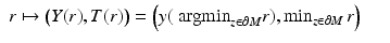
  . First, we show that we can identify in the set R(M) all the elements of the form r = r x ∈ R(M) where
  . To do this, we observe that r = r x with
  if and only if:
, where ω is the cut locus of M with respect to . First, we show that we can identify in the set R(M) all the elements of the form r = r x ∈ R(M) where . To do this, we observe that r = r x with if and only if:1.
 has a unique global minimum at some point
  ;
;
has a unique global minimum at some point ;2.
There is  having a unique global minimum at the same z and
  . This is equivalent to saying that there is y with
  having a unique global minimum at the same z and r x (z) < r y (z).
having a unique global minimum at the same z and . This is equivalent to saying that there is y with having a unique global minimum at the same z and r x (z) < r y (z).Thus, we can find  by choosing all those r ∈ R(M) for which the above conditions (1) and (2) are valid.
by choosing all those r ∈ R(M) for which the above conditions (1) and (2) are valid.Next, we choose a differentiable structure on  which makes the map
  a diffeomorphism. This can be done by introducing coordinates near each
  . In a sufficiently small neighborhood
  of r 0 the coordinates
 are well defined. These coordinates have the property that the map
  coincides with the boundary normal coordinates (17) and (18). When we choose the differential structure on
  that corresponds to these coordinates, the map
 is a diffeomorphism.
which makes the map a diffeomorphism. This can be done by introducing coordinates near each . In a sufficiently small neighborhood of r 0 the coordinates coincides with the boundary normal coordinates (17) and (18). When we choose the differential structure on that corresponds to these coordinates, the mapNext we construct the metric g R on R(M). Let  . As above, in a sufficiently small neighborhood W ⊂ R(M) of r 0, there are coordinates
  that correspond to the boundary normal coordinates. Let
  . We consider next the evaluation function
 where
where  . The inverse of
  is well defined in a neighborhood
  of (y 0, t 0), and thus we can define the function
 that satisfies
where  is the normal geodesic starting from the boundary point z(y) with coordinates
  and ν(y) is the interior unit normal vector at y.
. As above, in a sufficiently small neighborhood W ⊂ R(M) of r 0, there are coordinates that correspond to the boundary normal coordinates. Let . We consider next the evaluation function. The inverse of is well defined in a neighborhood of (y 0, t 0), and thus we can define the function(22)
is the normal geodesic starting from the boundary point z(y) with coordinates and ν(y) is the interior unit normal vector at y.Let now g R = R ∗ g be the push-forward of g to  . We denote its representation in X-coordinates by g jk (y, t). Since X corresponds to the boundary normal coordinates, the metric tensor satisfies
. We denote its representation in X-coordinates by g jk (y, t). Since X corresponds to the boundary normal coordinates, the metric tensor satisfiesConsider the function E w (y, t) as a function of (y, t) with a fixed w. Then its differential, dE w at point (y, t) defines a covector in  . Since the gradient of a distance function is a unit vector field, we see from (22) that
 Let us next fix a point (y 0, t 0) ∈ U. Varying the point
  , we obtain a set of covectors
  in the unit ball of
  which contains an open neighborhood of
  . This determines uniquely the tensor
  . Thus, we can construct the metric tensor in the boundary normal coordinates at arbitrary
  . This means that we can find the metric g R on
  when R(M) is given.
. Since the gradient of a distance function is a unit vector field, we see from (22) that, we obtain a set of covectors in the unit ball of which contains an open neighborhood of . This determines uniquely the tensor . Thus, we can construct the metric tensor in the boundary normal coordinates at arbitrary . This means that we can find the metric g R on when R(M) is given.To complete the reconstruction, we need to find the differentiable structure and the metric tensor near R(ω). Let  and
and  be such a point that
  . Let z 0 be some of the closest points of
  to the point x (0). Then there are points
  on
on  , given by
  , where
  are geodesics of
  and
and  are orthonormal vectors of
  with respect to metric
  and s 0 > 0 is sufficiently small, so that the distance functions
  ,
,  form local coordinates
  on M in some neighborhood of the point x (0) (we omit here the proof which can be found in [42, Lemma 2.14]).
and be such a point that . Let z 0 be some of the closest points of to the point x (0). Then there are points on , given by , where are geodesics of and are orthonormal vectors of with respect to metric and s 0 > 0 is sufficiently small, so that the distance functions , form local coordinates on M in some neighborhood of the point x (0) (we omit here the proof which can be found in [42, Lemma 2.14]).Let now W ⊂ R(M) be a neighborhood of r (0) and let  . Moreover, let
  and
and  . Let us next consider arbitrary points
  on
on  . Our aim is to verify whether the functions
 form smooth coordinates in V. As
  is dense on M and we have found topological structure of R(M) and constructed the metric g R on
  , we can choose
  such that
  in R(M). Let
  be the points for which
  . Now the function
  defines smooth coordinates near
  if and only if for functions
  , we have
Thus, for all  we can verify for any points
  whether the condition (23) is valid or not and this condition is valid for all
  if and only if the functions
 form smooth coordinates in V. Moreover, by the above reasoning, we know that any
  has some neighborhood W and some points
  for which the condition (23) is valid for all
  . By choosing such points, we find also near
  smooth coordinates
  which make the map R: M → R(M) a diffeomorphism near x (0).
. Moreover, let and . Let us next consider arbitrary points on . Our aim is to verify whether the functions form smooth coordinates in V. As is dense on M and we have found topological structure of R(M) and constructed the metric g R on , we can choose such that in R(M). Let be the points for which . Now the function defines smooth coordinates near if and only if for functions , we have(23)
we can verify for any points whether the condition (23) is valid or not and this condition is valid for all if and only if the functions form smooth coordinates in V. Moreover, by the above reasoning, we know that any has some neighborhood W and some points for which the condition (23) is valid for all . By choosing such points, we find also near smooth coordinates which make the map R: M → R(M) a diffeomorphism near x (0).Summarizing, we have constructed differentiable structure (i.e., local coordinates) on the whole set R(M), and this differentiable structure makes the map R: M → R(M) a diffeomorphism. Moreover, since the metric g R = R ∗ g is a smooth tensor, and we have found it in a dense subset  of R(M), we can continue it in the local coordinates. This gives us the metric g R on the whole R(M), which makes the map R: M → R(M) an isometric diffeomorphism.
of R(M), we can continue it in the local coordinates. This gives us the metric g R on the whole R(M), which makes the map R: M → R(M) an isometric diffeomorphism. In the above proof, the reconstruction of the metric tensor in the boundary normal coordinates can be considered as finding the image of the metric in the travel time coordinates.
Let us next consider the case when we have an unknown isotropic wave speed c(x) in a bounded domain  . We will assume that we are given the set
  and an abstract Riemannian manifold (M, g), which is isometric to
  endowed with its travel time metric corresponding to the wave speed c(x). Also, we assume that we are given a map
  , which gives the correspondence between the boundary points of
  and M. Next we show that it is then possible to find an embedding from the manifold M to
  which gives us the wave speed c(x) at each point
  . This construction is presented in detail, e.g., in [42].
. We will assume that we are given the set and an abstract Riemannian manifold (M, g), which is isometric to endowed with its travel time metric corresponding to the wave speed c(x). Also, we assume that we are given a map , which gives the correspondence between the boundary points of and M. Next we show that it is then possible to find an embedding from the manifold M to which gives us the wave speed c(x) at each point . This construction is presented in detail, e.g., in [42].For this end, we need first to reconstruct a function σ on M which corresponds to the function c(x)2 on  . This is done on the following lemma.
. This is done on the following lemma.Lemma 2.
Related posts:
 Segmentation with Shape Priors: Explicit Versus Implicit Representations
 Set Methods for Structural Inversion and Image Reconstruction
Stay updated, free articles. Join our Telegram channel

Full access? Get Clinical Tree


