“Pick your Poison”: The Arterial Spin Labeling Shopper’s Guide or which Method for which Application?

Hanzhang Lu

Matthias Günther

Xavier Golay

Susan R. Hopkins

Fritz Schick

Rebecca J. Theilmann

Petros Martirosian

Christina Schraml

Andreas Boss

Given the diversity of arterial spin label (ASL) implementations, the complexity of the acquisition and quantification schemes, and the confounding factors described in other chapters in this book, beginners who are interested in using ASL may find it difficult to know where to start. Different applications have different requirements in terms of cerebral blood flow (CBF) assessment. Some applications might have a strong emphasis on acquisition speed; another application may view the ability to carry out absolute quantification as the highest priority; others may put more considerations on the sensitivity of the approach. This chapter provides a recommendation for each of the major categories of ASL applications. Thus, depending on their specific application, the reader will at least have a good starting point to work with or to further tune the sequence.

The Use of ASL for Absolute Quantification of CBF

Complexity in ASL Quantification

Quantification of CBF with ASL is not a simple task. A number of parameters can affect the conversion from perfusion-weighted images (i.e., signal intensities modulated by blood flow, to quantitative numbers of CBF). Therefore, the important question for reliable quantification is, which parameters can be taken from literature and which parameters have to be measured, since they differ across subjects? There is no easy answer to this question, because the answer depends on the details of the study, such as pathology, age and sex of subjects, overall constitution of the patient, and many more.

Quantification of perfusion and other hemodynamic parameters rely on models that describe the dependency of the measured ASL signal from various parameters. The following sections examine typical models and explain which model can be used for which application.

As described in other chapters of this book, in ASL, the perfusion-weighted image is calculated by subtracting the image with the label preparation from the control data set, both acquired at time TI after preparation:

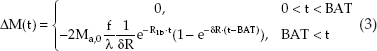
Depending on the time elapsed between labeling and reading out the data (i.e., the inflow time or historically the inversion time [TI]), the labeled blood magnetization will have traveled different ways down the arterial tree from the site of labeling toward the imaging slice. Thus, for a short TI, the arterial blood vessel might contribute more than at a later TI when the label has exchanged with the tissue. This makes it more complicated to quantify perfusion in pulsed arterial spin labeling (pASL). However, it also allows for true quantitative perfusion calculation and the possibility to acquire even more parameters describing hemodynamics. Later in this chapter, several formulas will be developed for the more complex behavior of the difference magnetization, ΔM, between label and control, but here a simpler expression is used without further derivation. The signal behavior of a voxel, where labeled magnetization is flowing in, can be described by the following equation:

Here, M_0b is the equilibrium magnetization of blood, R_1b (= 1/T_1b) is the relaxation rate of blood, δR is the difference in the relaxation rates R_1b and R_1t (= 1/T_1t) of blood and tissue, respectively, γ is the blood–brain partition coefficient, and f is perfusion. By assuming the value of some parameters (e.g., γ = 0.9 mL/g and R_1b = 1/1200 milliseconds for 1.5T), and measuring others, like M_0b and R_1t, it is possible to directly calculate perfusion f from Eq. 2. This already shows a fundamental challenge in quantification of ASL: there are several parameters, which influence the shape and size of the inflow curve. These are typically unknown and often replaced by literature values. This is no major problem as long as there is no major change over the population to be assessed. If there are changes, these have to be considered for reliable and comparable perfusion quantification. Eq. 2 is valid in cases of immediate inflow of labeled blood water directly after tagging. Although this might be a worthwhile assumption in some organs (depending on vessel geometry and positioning of labeling slabs), there often is a significant delay in the labeled blood bolus arrival in the brain. This delay is typically called the bolus arrival time (BAT), which is a very important parameter to
consider, since it varies from region to region within the same brain as well as across brains. This is even more so important in pathology, especially patients with cerebrovascular diseases.

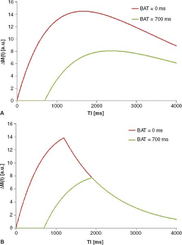FIGURE 22.1. Dependency of arterial spin labeling (ASL) signal on bolus arrival time (BAT): A: Both ASL signal curves have the same amount of perfusion, but the labeled blood bolus arrives at different points in time at the voxel. Large signal intensity changes are apparent because of the difference in label arrival as the label has already decayed with T₁. Thus, the ASL signal has a strong BAT dependence. B: The effect of quantitative imaging of perfusion using a single subtraction (QUIPSS II)-like saturation schemes. Due to the limitation of the labeled blood bolus to a fixed amount (by chopping off the tail end of the label), both ASL signal curves fall on top of each other after a certain inversion time (TI) (for TI >1900 milliseconds in this example). Imaging after TI (i.e., TI >1900 milliseconds in our example) leads to a direct correlation of the intensity of the ASL signal and perfusion, which does not depend on different BATs. Specifically, this requires that the BAT be less than TI minus the bolus length.

Incorporation of BAT into Eq. 2 yields the following equation:

Again, if all other parameters were known (including BAT), perfusion f could be calculated directly. Typically, this is not the case, since the BAT of different regions tends to differ in the same subject (e.g., BAT of gray and white matter tissue differ by some 400 milliseconds, with white matter tissue having a longer delay). Particularly in watershed areas, the BAT can be even higher than the value mentioned above; and BAT in the vascular territory supplied via the posterior circulation is different from that supplied through the anterior circulation.

Depending on how long the labeled blood needs to spins to reach the imaging voxel, the measured signal will vary tremendously (Fig. 22.1A), resulting in a large underestimation of the actual perfusion due to the decay of the label.

Quantitative Imaging of Perfusion Variants

An elegant solution to this strong dependency of measured perfusion on the BAT was presented by E. Wong et al.¹ and refined by Luh et al.² The basic idea of this approach is to limit the length of the labeled blood bolus by applying one quantitative imaging of perfusion (QUIPSS II) or multiple (Q2TIPS) saturation pulses caudally to the imaging slab at a given time before image acquisition commences (see Chapter 15 for more details on the technique). QUIPPSS II and Q2TIPS are essentially generating a sharp tail end of the bolus, which would otherwise be blurred out due to arrival time differences of the label into the imaging slab. QUIPSS II and Q2TIPS
differ mainly in how effective they are in trimming the bolus; Q2TIPS is usually more effective.

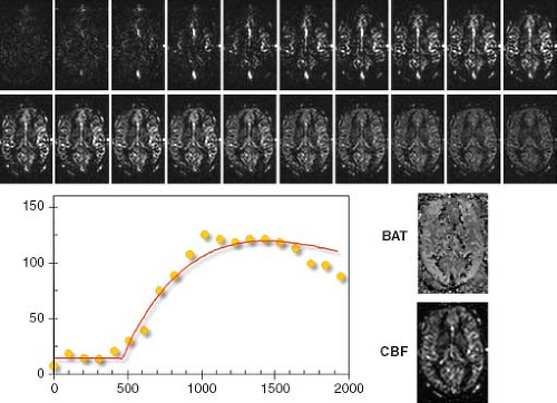FIGURE 22.2. Sampling of arterial spin labeling (ASL) signal curve: by varying the time delay, TI, between the time of labeling and image readout in pulsed ASL, the inflow of the labeled blood bolus can be measured. Modeling the characteristics of this inflow allows the extraction of parameters related to hemodynamics. The simplest model is a one-compartment model, which yields two parameters: perfusion or cerebral blood flow (CBF) and the bolus arrival time (BAT).

It was shown that, for certain parameter settings, the pASL difference signal is proportional to perfusion f.¹ It is then possible to calculate perfusion directly from data at a single inflow time. A major assumption or requirement of QUIPSS-based quantification approaches is that the complete labeled blood bolus (which was limited to a defined length by the saturation pulses) has flown into the voxel at the time of image acquisition. This must be fulfilled even for the latest BAT within the imaging region (Fig. 22.1B). To ensure this, the inflow time can be made very long. However, this will reduce the sensitivity of the method, since the labeled magnetization decays with (at least) the T₁ relaxation rate of blood. This means a tradeoff between long TI and accurate perfusion estimation has to be found. In young healthy human subjects, a good set of parameters can be found for reliable measurements. However, in sick and older patients, these requirements might not be fulfilled, and the perfusion quantification might yield incorrect values that either under- or overestimate perfusion.

Multitime Step (Sampling) Approach

A more reliable way of quantification of pASL experiments is the multi-TI approach. Sampling the inflow of tagged blood magnetization into the tissue of interest allows better determination of parameters of mathematical models, which are designed to describe a voxel of perfused tissue. Measuring the ASL signal curve at several inflow times allows estimation of parameters like BAT, which are otherwise assumed to be within a certain range (like in QUIPSS II variants) or taken from literature. Using this multi-TI approach, the parameters can then be estimated on a per-voxel basis to describe the measured signal behavior in the best way. The models used can be arbitrarily complicated depending on the level of complexity and the number of parameters involved. However, typically robustness and reliability decrease with increasing complexity of the model.

Figure 22.2 shows a typically ASL time series by acquiring data 20 different inflow times that are spaced 100 milliseconds apart. The red curve shows the optimal fit of Eq. 3 to a single voxel. Here, CBF and BAT maps of the respective slice show the regional variance of these two parameters.

The multi-TI approach is the most powerful method of ASL data analysis, because it allows for direct (and voxel-wise) estimation of parameters describing the underlying tissue. A critical point, however, is the robust extraction of parameters for a given data set and model used. Most often, nonlinear optimization approaches are used, such as the Levenberg-Marquardt. Recently, a more robust way of parameter extraction, using Bayesian analysis, was described.³ This approach incorporates prior information about the parameters based on physiologic knowledge, thus enabling a more robust estimation of parameters compared to previous methods.

A considerable disadvantage of the acquisition of an ASL time series study is that it is rather time consuming; each time step has to be acquired separately. Using a Look-Locker approach allows acquisition of more than one inflow time after a single preparation.⁴^,⁵^,⁶ This approach is powerful for sampling arterial inflow, but caution must be made so as not to fully saturate the blood flowing into the microvasculature. As a result, a smaller flip angle (e.g., 15 to 35 degrees) is recommended, although this would
reduce the per-image signal-to-noise ratio (SNR). The time that the Look-Locker approach saves can be used to increase the number of averages to regain SNR.

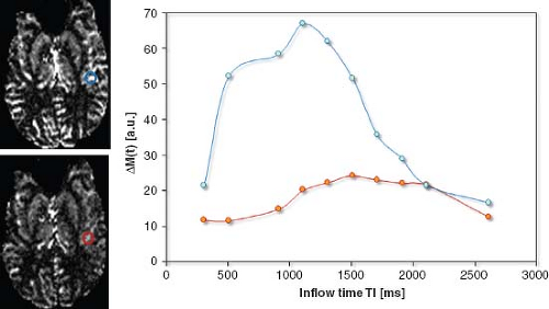FIGURE 22.3. Suppression of intra-arterial blood signal by use of crusher gradient pulses (small diffusion-weighting with b value of 10 s/mm²). Note that the efficiency of crushers in suppressing vessel signal depends on the relationship between flow and gradient directions.

In some regions, the labeled blood signal in larger arteries (rather than capillaries and tissue) will dominate perfusion values acquired by ASL. Ye et al.⁷ proposed the use of bipolar crusher gradients to dephase the (moving blood) signal from the large feeding arteries in continuous arterial spin labeling (CASL) experiments. This was also adapted for pASL sequences.⁸ Figure 22.3 shows the effect of flow-crushing gradient pulses on the ASL signal at several inflow times. The blue curve clearly exhibits a large amount of arterial signal contribution, which can be reduced by these spoiler gradient pulses. A problem of this approach is the difficulty in accurately estimating the optimal setting for the crusher gradients to only dephase spins flowing in larger vessels without attenuating the signal of blood spins contributing to local CBF. (Notice that with increasing gradient strength or duration of these crusher gradients, more diffusion weighting is added.)

An elegant approach to use flow-crushing gradients to more accurately quantify perfusion is the model-free approach by Petersen et al.⁵ Here, two time series, with and without crusher gradients, are used to estimate the arterial input function for each voxel and estimate perfusion without the need for explicit modeling. Specifically, the time series without the crushers contains arterial and tissue signal, while the time series with the crusher contains tissue signal only. Thus, subtracting the results of the time series with crushers on from that without crushers will yield the arterial signal only and therefore the arterial input function.

Be cognizant that the Look-Locker approach drives the magnetization of tissue and arterial label into a different steady state than what would be seen with a multi-TI experiment. With Look-Locker, spins recover with a pseudo-T₁ time, which differs from the normal T₁ relaxation time, and the label and control converge to a similar steady state, which depends on the repeat rate and flip angle of the Look-Locker readout and in turn reduces the label efficiency.

Arterial signal contribution in pASL time series can also be estimated by a postprocessing algorithm, which incorporates the macrovascular compartment into the model.³

Another relevant issue is the estimation of M_a,0 and also T₁ relaxation time of tissue and blood. Here, several approaches exist. In cases of a multi-TI acquisition, the most common way is to use the time-series data of the ASL acquisition, but instead of subtracting the two data sets according to Eq. 1, only the control data are used. For different inflow or inversion times, TI, the signal follows an inversion (or saturation) recovery curve, allowing the extraction of M₀ and T₁. Unfortunately, modern ASL sequences typically use background suppression to null out the signal of stationary tissue, as any patient motion may easily dominate the signal difference between label and control and would swamp the effect of perfusion that emanates from the ∼2% (in brain) capillary blood volume. Due to the absence of any significantly measureable tissue signal, these sequences will not allow performance of this type of mutual parameter estimation. Therefore, an additional, multipoint saturation or inversion recovery acquisition has to be used, which adds extra scan time.

Application of ASL in Cerebrovascular Diseases

Perfusion and Cerebrovascular Diseases

Perfusion-weighted imaging (PWI) plays an important role in the diagnosis of potentially salvageable tissue in acute stroke because of the difference in the timing of signal
changes between PWI and diffusion-weighted imaging.⁹ Indeed, the irreversibly infarcted tissue is usually assessed using the signal from the latter, as high signal on diffusion-weighted images represents reduced water diffusion and impaired tissue metabolism. It is a very good and conspicuous marker of irreversible damage. There is strong evidence that tissue with an apparent diffusion coefficient of less than 550 to 650 × 10⁻⁶ mm²/s is irreversibly damaged. on the other hand, CBF really defines the extent of hypoperfusion, and PWI will therefore provide a more subtle description of the evolution of the acute ischemic event. Generally, the brain’s perfusion level is about 50 mL/min/100 g tissue, and although it can compensate for loss of perfusion pressure, following an acute obstruction of a feeding vessel through autoregulatory processes, such as arteriolar vasodilatation, there is a tipping point in the perfusion pressure below which the tissue will go into energy failure and cytotoxic edema leading to infarction.

Some evidence suggested that gray matter CBF that is 40% below its normal value can be tolerated indefinitely, and this flow range is often referred to as benign oligemia.¹⁰ Below a certain level, the appearance of irreversible tissue damages will depend on the duration of the insult. In this context, the duration of the ischemic event also plays a key role. Notice that there is currently an ongoing debate in the stroke neurology community about the validity of naming convention for terms, such as infarct core, penumbra, or benign oligemia, their exact definitions, and whether or not perfusion thresholds can be used as simple surrogates. For more information, see Chapters 30 and 31.

Acute ischemic attacks are sometimes preceded by transient ischemic attack, which might represent a clinical challenge for its detection because of the lack of a clear imaging signature as opposed to stroke. Finally, chronic hypoperfusion states associated with large artery disease and complicated neurovascular pathologies such as Moyamoya disease might also generally benefit from PWI.

ASL in Cerebrovascular Diseases

As mentioned previously, ASL using multiple inversion times TI is the most powerful way of determining various perfusion parameters. This becomes very important for cerebrovascular diseases, both for stroke and atherosclerotic diseases, as timing parameters, such as BAT, have been shown to be as important as the CBF (f) itself.¹¹ Indeed, so far, the preferred method for assessing perfusion impairments in stroke is based on the measurement of timing parameters such as the mean transit time (MTT = cerebral blood volume [CBV]/CBF)¹² or time to maximum (Tmax),¹³ an arterial input function–normalized bolus arrival time assessed using dynamic susceptibility contrast (DSC) MRI. Those parameters usually show a much clearer separation between healthy and diseased tissue than the conventional physiologic parameter CBF, despite CBF’s role in the definition of oligemic and ischemic areas. More importantly, in healthy brain there is little contrast between gray and white matter, rendering those time-parameter maps relatively flat and, therefore, increasing the conspicuity of areas of hemodynamic abnormalities.

Because of the nature of the contrast mechanism used in ASL, for which arterial water is noninvasively labeled and used as intrinsic tracer, the assessment of the entire CBV compartment is close to impossible. In fact, there is no or very little difference between intra- and extravascular labeled arterial water spins before and after their exchange with the tissue of interest, with the exception of subtle differences in relaxation times.¹⁴^,¹⁵ As such, conventional ASL cannot measure total CBV, and therefore cannot assess the MTT. However, Look-Locker sampling schemes or similar multi-TI acquisitions provide very accurate measurements of BAT on a per-pixel basis. These measurements are much more precise than the ones obtained by DSC. This is because of the better temporal resolution, which comes mainly from the ability to repeat the measurements with multiple inversion times. For example, assessment of BAT using ASL has been capable to highlight the border-zone areas between main perfusion territories even in healthy volunteers, based on subtle differences on arrival times.¹⁶ The greater sensitivity of ASL to bolus arrival can be helpful in subtle cerebrovascular abnormalities, such as for transient ischemic attack. However, a major shortcoming of ASL-based measurements in patients suffering from acute stroke, for example, is that clinically relevant areas have usually Tmax times of 4 to 6 seconds or longer, which is beyond the lifetime of the ASL.

Note that multitime point pASL is not the only possible ASL sequence to be used in atherosclerotic and embolic diseases. Pseudo-CASL (pCASL) or CASL sequences could also be used in such diseases. The main advantage of these continuous labeling sequences, as explained in Chapters 15 and 17, is mostly the increased SNR in the normal (or nonischemic) tissue as they are supposed to provide measurements in the steady state. Under those circumstances, a reduced perfusion signal in the infarcted tissue might be related independently to either a reduced perfusion rate or a delayed arrival of the blood to the tissue. Although this looks like a big disadvantage at first, the fact that both reduced perfusion and delayed arrival time might be used as marker of at-risk tissue makes those sequences interesting in radiological practice, as it will provide a very quick and conspicuous way to separate healthy from diseased tissue.¹⁷^,¹⁸ In addition, the presence of arterial signal in the large vessels surrounding the infarcted area is a very clear indication of the presence of collateral perfusion, thereby further enhancing the clinical information
present in these images.¹⁷ This, however, comes at the cost of a reduced or biased quantitative information. In this context, it is interesting to note that this dependency on arrival times of CASL and pCASL has been used for the definition of global cerebrovascular burden¹⁹ and has even been used to allow for a rough assessment of delayed arrival time using successive CASL measurements with and without use of vascular crushers flow encoding arterial spin tagging.²⁰

FIGURE 22.4. Magnetic resonance angiography showing a severe stenosis in a patient’s distal right internal carotid artery (ICA) and middle cerebral artery (MCA) with substantially decreased perfusion of the right MCA perfusion territories as evidenced by the lack of perfusion signal in this area. Only some residual perfusion signal of the right ICA is still visible (shown in red) surrounding the internal border zone infarcts in the deep white matter. Shown in green is the perfusion territory of the left ICA, whereas the territory supplied by the vertebrobasilar system is shown in blue.

Collateral Perfusion

One of the most important mechanisms the brain has to prevent malignant progression of an ischemic attack is the possibility to change the distribution of blood via collateral perfusion. Originally, collateral perfusion was assessed using invasive dynamic subtraction angiography in most stroke cases; however, the advent of modern imaging techniques made diagnostic dynamic subtraction angiography for acute ischemic stroke obsolete. Yet, the possibility to clearly assess the blood paths through the brain following obstruction of a major artery was lost in the process, as conventional PWI relies on the global injection of contrast agent, without access to individual labeling of arteries.

This is, however, not the case for ASL, which may provide for independent labeling of single arteries. In fact, most ASL techniques can be made to label selective individual arteries. These methods have been published under various names, such as perfusion territory imaging,²¹ regional perfusion imaging,²² selective²³ or territorial ASL,²⁴ or vessel-selective ASL,²⁵ but they are all based on similar principles, as illustrated in Figure 22.4. Many approaches have been proposed, and the simplest is probably the use of selective labeling of an individual artery using a separate coil.²¹ The main drawback of this method is that it requires extra hardware and limits the acquisition to arteries easily accessible in the neck. A more clinically feasible approach is to use an angulated pulsed labeling slab to include only a single artery at a time. The labeling pulse will, however, in most cases intersect with the tissue of interest, and a strong saturation preparation needs to be applied in the tissue of interest to avoid direct tissue inversion. This is difficult to achieve at higher field strengths.²⁶ Thus, a careful, time of flight magnetic resonance angiography–based planning of the labeling pulse needs to be performed.²² It is, however, a relatively complicated procedure, and more recent methods, based on CASL²⁷ and pCASL,²⁵ are much easier to implement as the selection of vessels can be done blindly and without the need for careful angulation planning. In the pCASL-based method, selective labeling of individual arteries is achieved by adding additional gradients to the labeling module of the pulse sequence. When this acquisition scheme is combined with postprocessing, involving an algebraic combination of several scans, vessel-specific perfusion maps can be obtained.

Using these methods, several studies have shown the clinical potential of ASL to assess collateral perfusion.²⁸ Thus far, most clinical applications of region-selective ASL have been for the assessment of the distribution of blood flow in large vessel disease,²⁴^,²⁹^,³⁰ the estimation of perfusion territories after bypass
surgery or endarterectomy,³¹^,³²^,³³^,³⁴ and the measurement of cerebrovascular reactivity.¹⁶^,³⁵^,³⁶

Application of ASL in Psychiatric Disorders

Rationale of Applying ASL Magnetic Resonance Imaging in Psychiatric Disorders

Although most psychiatric disorders do not have an etiology of vascular origin, measurement of CBF is still of great interest to researchers and clinicians in this field, especially as direct mapping of neural activity in awake humans has proven difficult with current technologies. Here, CBF serves as a surrogate marker for the underlying neural activity based on the assumptions that neural activity and CBF are tightly coupled³⁷ and that a brain region with a higher (or lower) neural activity should be accompanied by a higher (or lower) CBF.

This relationship of neurovascular coupling was first proposed more than a century ago³⁷ and is generally considered valid in individuals who do not have vascular diseases. A caveat is that cautions should be used when interpreting CBF data from patients who are currently on or have recently received medications. Many medications have a vasoactive effect, thus this may alter blood flow independent of the effect of the disease.³⁸^,³⁹ Therefore, it is important to distinguish vascular from neuronal origins when interpreting CBF changes. One notion that may be useful in this regard is that vascular effects of medications are most likely present throughout the whole brain, whereas neural effects due to disease may be more localized to specific brain regions or specific types of neurotransmitters. Therefore, by evaluating local CBF changes in the context of global change, it is in principle feasible to isolate the neural changes from vascular changes.

Unlike studies of neurologic diseases, where the use of exogenous contrast agent is relatively routine,¹¹^,⁴⁰ psychiatrists are more used to noncontrast-based magnetic resonance imaging (MRI) techniques, and there can be concerns as to whether it is justifiable to apply contrast agent in these patients. Thus, ASL is often favored over DSC or dynamic contrast-enhanced (DCE) MRI techniques. As a result, there is growing interest among researchers to use ASL to better understand the mechanisms of psychiatric disorders.

Factors to Consider When Picking an ASL Protocol for Psychiatric Studies

Signal stability is the most important factor in psychiatric studies using ASL. Unlike neurologic diseases, changes in CBF in psychiatric studies are expected to be small.⁴¹^,⁴²^,⁴³ In order to detect a difference of this magnitude, the signal needs to be sufficiently stable. Otherwise, the sample size needed to detect a difference will be beyond manageable.

Spatial coverage is also an important consideration. The brain regions that are potentially involved in psychiatric diseases are often unclear, and there are no obvious lesion regions to focus on. Thus, with few exceptions, it is usually desirable to cover the entire brain in a scan.

Mapping of arterial transit time is considered optional. As mentioned, psychiatric disorders are usually not of vascular origin. Thus, heterogeneity in arterial transit time across brain regions or across individuals is not a major concern. Therefore, a single postlabeling delay time is considered sufficient in these studies.

There can be a misconception that absolute quantification of CBF (milliliters/100 grams/minute) is always more useful than a relative value (for example, relative to the whole brain or relative to a reference region such as cerebellum). However, in practice the absolute CBF value is not necessary more sensitive in all situations. In the case of psychiatric diseases, relative CBF is expected to be a more useful marker. The reason is that absolute CBF is affected by many nondisease-related factors, such as breathing pattern, consumption of caffeine, and time of the day. As a result, normal variations in absolute CBF are often large. on the other hand, the factors mentioned previously are largely removed when relative CBF is calculated using a reference region or whole brain for normalization, because these factors affect the CBF in a global manner instead of a region-specific manner.⁴⁴ Consequently, normal variations in relative CBF could be several-fold smaller.

ASL Protocol Recommendations in Typical Psychiatric Applications

Type of ASL Sequences

Previous theoretical and experimental investigations have established that CASL provides a higher sensitivity compared to pASL.⁴⁵ However, the limitation of the conventional CASL method was that a special transmission coil is needed in order to ensure that the power used is within the guidelines. Fortunately, a recently revised version of cASL, pCASL, maintains the advantages of CASL but allows the implementation using standard hardware.⁴⁶ Thus, it is recommended that the pCASL labeling scheme be considered whenever possible.

Labeling Duration

The labeling duration should be considered in the context of SNR per unit scan time. In principle, longer labeling duration would allow more labeled spins to reach the brain tissue, thus generating a greater ASL signal. However, since the labeling effect decays exponentially with the T₁ relaxation time of blood (or tissue in case the
spins have left the capillaries already), the ASL signal increases only marginally beyond a certain labeling duration. on the other hand, a longer labeling duration will usually result in a longer repetition time (TR) and, thus, the scan duration also becomes longer. Therefore, a moderate labeling duration of 1500 to 2000 milliseconds is recommended in practice.

Postlabeling Delay

In addition to CBF, ASL signal can also be sensitive to the BAT parameter (i.e., the time it takes for the labeled blood spins to reach the imaging voxel). In certain neurologic diseases, such as stroke, the arterial transit time itself is a useful marker for disease severity. In psychiatric disorders, on the other hand, the arterial transit time is expected to reflect interindividual heterogeneity only and does not contain disease-specific information. Thus, efforts should be made to reduce the influence of arterial transit time on ASL signal. A pos-labeling delay with a value greater than BAT can be placed between the labeling pulses and the image acquisition to ensure all labeled spins reach their “destination.” Previous studies have reported that the arterial transit time is in the range of 500 to 1200 milliseconds, depending on the locations of the labeling plane and imaging slice.⁷^,⁴⁷^,⁴⁸ Thus, the postlabeling delay time should be chosen to be greater than these values. In practice, a slightly longer delay time is often used in order to account for potential heterogeneities in transit time across voxels. on the other hand, an excessively long postlabeling delay time is not desirable either, because the delay does result in a time-dependent reduction in ASL signal (due to T₁ recovery of the label). With all factors considered, a postlabeling delay of 1200 to 1800 milliseconds is recommended for psychiatric ASL applications.

Image Acquisition and Background Suppression

Two common schemes used in ASL image acquisition are two-dimensional (2D) multislice echo-planar imaging (EPI)⁴⁹ and 3D gradient and spin echo (GRASE).⁵⁰^,⁵¹ The 2D EPI scheme acquires images in a slice-by-slice manner, usually from bottom to top. Because different slices are acquired at different times relative to the time when the arterial labeling pulses are played out (the 2D-EPI readout for one slice is, depending on matrix size, several tens of milliseconds), the actual postlabeling delay is slightly different for different slices. For example, if the nominal postlabeling delay is 1800 milliseconds, then only the first slice was acquired at 1800 milliseconds. The second slice is acquired at 30 to 40 milliseconds later, which is the time it takes to excite and acquire one slice, and so on for later slices. That is, the last slice of the brain might be acquired with a postlabeling delay of as long as 3000 milliseconds, if one assumes a total of 31 slices. This creates a relatively large heterogeneity in postlabeling delay times and associated image contrast. Conversely, the advantage of the 3D GRASE scheme is that all slices will be acquired at the same time and do not have differences in postlabel delay times (at least not for the contrast determining region of the k-space). Another advantage of a 3D acquisition is that it usually offers a greater SNR than 2D acquisition. Lastly, 3D acquisitions allow one to take full advantage of a background suppression scheme that uses inversion pulses to suppress static tissue signal as the contrast-determining k-space center is acquired when background nulling is most optimal. When applied to 2D acquisitions, background suppression produces a new problem in that signal intensities in different slices are unequally scaled (due to different effective inversion times for each slice), making it difficult to perform image realignment due to subject motion. The 3D acquisition does not suffer from this problem because signals are equally scaled across slices. When using background suppression, a noteworthy point is that, unless complex images with both magnitude and phase information are obtained, it is important to ensure that the longitudinal magnetization is positive at the time of image readout. If the total magnetization is still inverted, the labeled scan will yield a signal magnitude that is greater than the control scan. This, in turn, would result in an apparently erroneous negative CBF value. Therefore, it is recommended to adjust the background suppression inversion time so that the magnetization is 5% to 10% of the equilibrium value to account for possible heterogeneities in tissue T₁ relaxation times across the brain.

As mentioned previously, whole brain coverage is often desired for psychiatric studies. This means that about 30 slices (head-to-foot direction) are needed for the scan. Unfortunately, this number of slices is considered beyond the capacity of single-shot 3D GRASE, because it would result in an excessively long (>400 milliseconds) echo-train length and associated, severe blurring along the phase-encode direction that is read out slowest (usually slice direction). As a result, a two-shot, three-shot, or four-shot 3D GRASE should be considered in which each shot acquires only part of the k-space data.⁵² The multishot acquisition will potentially make the sequence more sensitive to motion but will improve the point-spread function along the accelerated read out direction (usually the slice direction). Note that background suppression can alleviate the motion problem to some extent. Taking all factors into consideration, it is recommended to use whole brain, multishot 3D GRASE with background suppression for ASL acquisitions to study psychiatric disorders.

Number of Averages

The number of averages used in an ASL scan depends on the desired SNR as well as the amount of time available. Figure 22.5 shows CBF maps as a function of number of
averages. It can be seen that an average of four or greater can usually yield a relatively stable CBF map.

FIGURE 22.5. Arterial spin labeling (ASL) image quality as a function of the number of averages. The images were acquired using pseudo-continuous ASL with multishot three dimensional gradient and spin echo acquisition with background suppression. Four shots per image (repetition time [TR] = 3.8 s). The scan duration for each average is 30 seconds.

Only gold members can continue reading. Log In or Register to continue