Principles of Elastography
2.1 Introduction
Elastography, or elasticity imaging, is a newer ultrasound imaging modality that can provide clinically useful information about tissue stiffness (rather than anatomy), which was previously unavailable. Palpation has been used to assess stiffness to evaluate for malignancies for at least a thousand years.1 Ultrasound elastography can be considered the imaging equivalent of clinical palpation as it can quantify the stiffness of a lesion, which was previously judged only subjectively by physical examination. With the addition of elastography, we now have three ultrasound modes: B-mode which evaluates acoustic impedance and provides anatomical information; Doppler which evaluates motion and provides vascular flow information; and elastography which evaluates mechanical properties and provides tissue stiffness information.
There are two major types of ultrasound elastography, strain elastography (SE) and shear wave elastography (SWE).2 SE produces an image based on how tissues respond to a displacement force from an external transducer, an acoustic radiation force impulse (ARFI), or from a patient source (breathing or heartbeat). This allows for a qualitative assessment of how stiff the lesion is compared to surrounding tissues in the field of view (FOV). With SE, the exact stiffness is not known, only how stiff one tissue is compared to other types of tissue in the field of view (FOV). SWE utilizes acoustic radiation force impulse (ARFI), often called a “push pulse,” as the compressive force. The natural sequel to this push pulse is the production of shear waves. Shear wave speeds are measured using conventional B-mode imaging to identify the tissue displacement caused by the shear waves. The shear wave speed (SWS) varies with tissue stiffness, with slow SWSs in softer tissue and higher SWSs in stiffer tissue. Therefore, the SWS allows for quantification of tissue stiffness.
Most vendors offer multiple elastographic choices depending on the transducer. A detailed list of each vendor and what they offer can be found in the World Federation for Ultrasound in Medicine and Biology (WFUMB) guidelines.
Here we present a brief discussion of the principles of ultrasound elastography. The goal of this chapter is to provide a very clinically oriented overview, and not a rigorous discussion, of the physics of ultrasound elastography. A detailed discussion of the principles of elastography can be found in other publications.3,4 Here we present a brief review of the basic principles behind approved ultrasound elastography techniques that are used for performing clinical exams.
2.2 Strain Elastography
SE determines the relative strain on, or elasticity of, tissue within an FOV.2 The more an object deforms when a force is applied, the higher the strain and the softer the object; the less an object deforms when a force is applied, the lower the strain and the stiffer the object. To determine the strain on a tissue or lesion, an external force is applied and how the tissue changes shape is monitored. This force can vary from minimal, such as patient breathing or his/her heart beating, to moderate rhythmic force generated by transducer movement. For example, if we had an almond within some gelatin (▶ Fig. 2.1) and pushed down on the gelatin, the gelatin would deform significantly indicating it has high strain and is therefore soft. However, the almond would not deform indicating it has low strain and is therefore stiff.
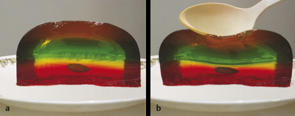
Fig. 2.1 A simplified model of the principle of strain elastography. (a) Consider an almond in gelatin. (b)If we apply a stress, such as compressing the gelatin with a spoon, the gelatin changes shape because it is soft (more strain), while the almond does not change shape because it is stiff (less strain). The ultrasound strain system compares the frame-to-frame changes of tissue when the tissue is compressed and released. Tissues that deform the most are considered soft, while those that deform the least are considered stiff.
SE is performed on standard ultrasound equipment using specific software that evaluates the frame-to-frame differences in deformation in tissue when a force (stress) is applied. The force can be from patient movement (such as breathing or heartbeat) or from external compression due to rhythmic motion of the ultrasound transducer or ARFI pulses.2 In SE the value of the absolute strain modulus (Young’s modulus)—a numerical value quantifying the stiffness—cannot be calculated because the amount of the force cannot be accurately determined. The real-time SE image is displayed with a scale based on the relative strain (or stiffness) of the tissues within the FOV. Therefore, if the types of tissue in the FOV differ from one display map to the next, a different dynamic range of stiffness values will be used in the display map leading to a different “color” for the same tissue.
2.2.1 Application of Stress
The technique required to obtain the optimal SE images varies with the algorithm used by the manufacturer of the system.2 For SE, the amount of external displacement needed varies depending on the algorithm used; presently, approved systems require from a 0.1 to 3.0% displacement for optimal elastograms. With some systems very little if any manual compression–release is needed, while with others a rhythmic compression-release cycle is required. With experience and practice the compression-release technique for a specific system to obtain optimal image quality can be learned. Applying too much compression–release will result in image noise, while not applying enough compression-release will result in no image being obtained. Learning the “sweet spot” for the equipment being used is critical for optimal images. The amount of displacement and the frequency of displacement significantly affect the quality of the elastogram.
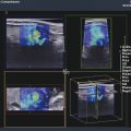
Some vendors have a visual scale that helps to confirm that the optimal compression-release and frequency are applied. This could be displayed via a quality measure, usually a number from 0, very poor, to 100, optimal. The information can also be displayed as a bar that changes size with the image quality, with a small bar as suboptimal and a large bar as optimal (▶ Fig. 2.2). Some systems provide a display that plots the displacement and frequency of the applied force and has optimal displacement and frequency displayed. The user can then monitor the displacement and frequency applied and try to optimize the stress for that system (▶ Fig. 2.3).
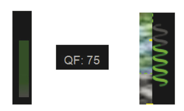
Fig. 2.2 Several of the numerical or visual scales used to display the amount of compression–release being applied. When the appropriate amount of compression–release is applied, the scales are maximized. If the compression–release is either too great or not sufficient, the scale will be smaller. For some systems, maximizing the green bar height confirms adequate compression-release, while in others increasing the number confirms adequate compression-release.

Fig. 2.3 Monitor display of the compression–release in real-time, available on some systems. In this example, the two central dotted lines are the optimal degree of displacement. The purple box on the right displays the displacement and frequency of the applied stress in yellow. The optimum displacement and frequency occur when the yellow just fills the purple box. This real-time feedback allows the sonologist the ability to optimize the elastogram while scanning.
When learning how to perform SE with the manual displacement method, it is helpful to practice varying the amount of displacement and the frequency of displacement while watching the display bar, quality measure, confidence bar, or displacement plots. You can identify the appropriate technique required by experimenting with your displacement technique and using the color bar or number to identify the optimal technique for the system you are using. When the appropriate technique is used, the elastogram should be similar on all frames. Other factors are important in obtaining optimal images so a high quality factor does not guarantee optimal images. The lesion should appear similar on all frames of the SE clip. If not, there is non-uniform displacement of the lesion during scanning or unacceptable precompression is being applied.
The algorithm used in SE requires the strain changes be measured in a lesion that remains within the imaging plane. Thus, the same location in the lesion needs to remain in the imaging plane during the entire compression-release cycle (▶ Fig. 2.4). Monitoring of the B-mode image to confirm that the lesion is only displaced in depth (not in- and out-of-plane) during scanning and only moving axially in the FOV will allow for optimal images. Positioning of the patient so that breathing or other motion, such as that from the heartbeat, is parallel to the transducer will help. With the SE techniques that involve displacement surveying an organ cannot be performed, as scanning must be done in one stationary position.
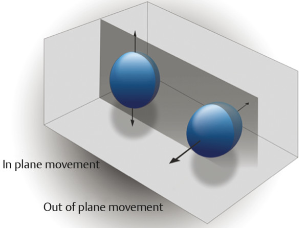
Fig. 2.4 When performing strain elastography, it is important that the same image plane through a lesion be maintained during data acquisition. The dark gray plane corresponds to the ultrasound beam. An optimal elastogram is obtained with only in-plane movement of the lesion. Out-of-plane movement may result in inaccurate elastography results.
Also the displacement needs to be applied uniformly to the tissues in the field of view. If the transducer is heel-toed, the stress applied will be different throughout the image and inaccurate results will be obtained. Examples of properly and improperly applied displacement are shown in ▶ Fig. 2.5. The degree of displacement can be displayed in a “motion map” using a color scale to indicate the amount of stress applied to the tissue. This technique is not yet clinically available but would be an excellent training tool. In the ideal case, the color of the motion map would be uniform throughout (▶ Fig. 2.5a). However, usually horizontal zones of color are displayed because the displacement often varies with tissue depth. Ideally when comparing tissues (such as in strain ratios discussed below), the same displacement should be applied to the tissues being compared to ensure accurate measurements.
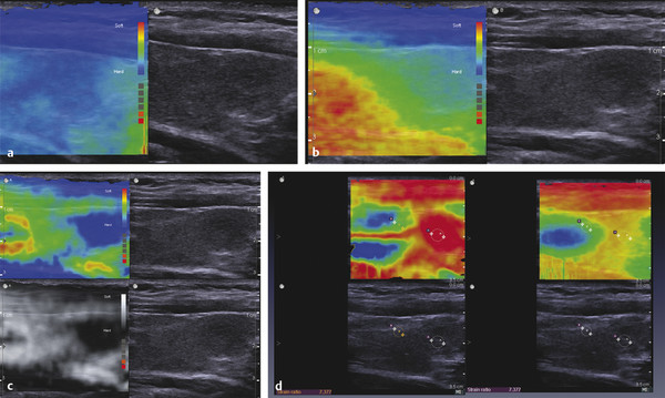
Fig. 2.5 A display of the distribution of stress in real-time, which has been developed but is not yet clinically available. In this display, the amount of stress in each region of the FOV is color-coded based on the amount of tissue displacement. A uniform blue display would be the optimal application of stress. Usually the stress varies with tissue depth (vertically) (a) but should be uniform at the same tissue depth (horizontally) in the image. When obtaining strain ratios, measurements should be taken at the same tissue depth; that is, within the same color. If the transducer is heel-toed, the stress applied is not uniform (b), with the stress being higher at one side of the image compared to the other. The map also allows one to visualize stress that may be coming from a different source, such as the carotid artery pulsations. The red and yellow ring in the left side of the image (c) is caused by carotid artery pulsations in this SE image of the thyroid. If too much stress is applied, the motion map will display a significant amount of red in the image (d). This real-time technique can be used as a training method for learning how to apply the stress to obtain the optimal images.
SE images are generated from the raw data of the B-mode images. Therefore it is important to obtain quality B-mode images before activating the SE mode. Find a scanning window that allows for stable positioning of the transducer during the compression-release cycle. If there are areas of shadowing they degrade the accuracy of the elastogram. Placing the palm of your hand on the patient helps stabilize the transducer and allows for more sensitive movements (▶ Fig. 2.6).
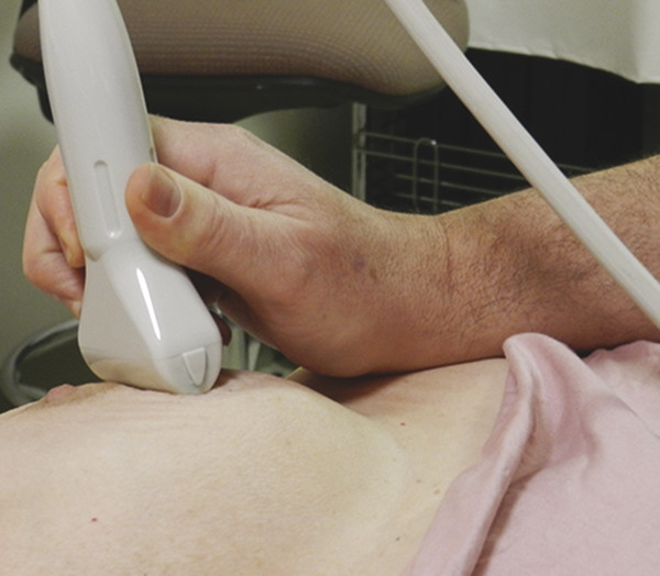
Fig. 2.6 Patient and transducer positioning for obtaining optimal elastograms. The patient should be positioned so that the imaging plane is the same as plane of patient’s respiration movements. Placing the palm of the scanning hand on the patient will help stabilize the transducer and improve the ability to execute fine movements.
2.2.2 Display of SE Results
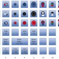
▶ Fig. 2.7 demonstrates a simplified explanation of how the mapping of SE data is performed on most systems. The boxes on the left represent tissue identified on B-mode imaging before the application of any compressive force. The boxes in the middle represent the deformation of the same tissue on B-mode imaging after the application of compressive force. The tissues that do not change shape are very stiff, while those that are soft change size based on their relative stiffness. The strain elastography algorithm evaluates the relative changes in size of the tissues and assigns a color (or shade of gray) based on the distribution of the size changes in the image. In our example in ▶ Fig. 2.7a, the tissue that does not change shape at all is color-coded black as it is the stiffest of all the tissue being evaluated. The lower box changes the most and is therefore the softest and is color-coded white. The tissue in between these extremes is given a shade of gray corresponding to the amount of change in the tissue; darker gray if stiffer and lighter gray if softer. However, if we did not include the stiffest tissue in field of view (FOV) of ▶ Fig. 2.7a, different color-coding of the other tissues will result, as in ▶ Fig. 2.7b. Note that the coloring of the first three tissues has changed because the second tissue is now the stiffest and is therefore coded black. Thus, the range of stiffness values is dynamic; it changes depending on the tissues present in the FOV. Thus, the “color” of a tissue will vary depending on the FOV.
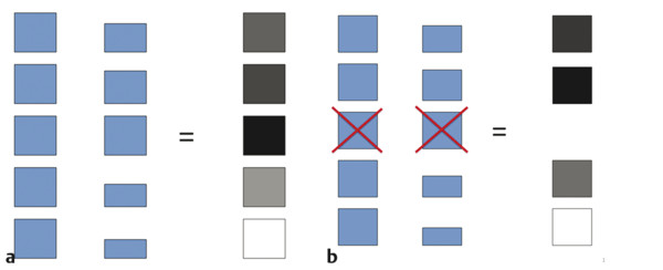
Fig. 2.7 Changes that occur in the color-coding of the pixels in the elastogram based on changes in the field of view (FOV). In these diagrams, the boxes on the left depict different tissues within the field of view. When compression is applied, the boxes change shape based on the stiffness of the tissue (center column). The box that changes shape the most is color-coded white, while the box that changes the least is color-coded black (right column). The boxes whose changes are between these two extremes are color-coded in shades of gray based on the amount of change they experience (a). If the FOV is changed (b) and the stiffest tissue in (a) is not included, the color mapping changes, with the second box now the stiffest and therefore being color-coded black. The dynamic range of the color-coding changes and the first and fourth tissues are now color-coded with darker shades of gray.
Therefore, if the same variety of tissues are included in each image acquired, a more relatively constant color display will be obtained for each tissue. For example, in breast SE, if a portion of the pectoralis muscle, glandular tissue, and some fat are included in the FOV each time, a more consistent color (or grayscale) depiction of these tissues will be obtained across images. The fat will be the softest tissue coding white and the pectoralis muscle will be the stiffest tissue (if a cancer is not present) coding black. The color scale (or dynamic range of stiffness values) will be fairly constant as the stiffness of fat and pectoralis muscle are very constant between patients and within a patient. However, if a breast cancer, which is stiffer than pectoralis muscle, is present within the FOV, it will be the stiffest tissue and will be black, with most other tissues being displayed as white or light gray.
Results can be displayed in grayscale or with various color displays; which is preferred is often determined by the user’s exposure to elastography and preference in interpretation. The choice of display map is a postprocessing function, and, on most equipment, the map can be changed when the image is frozen. The default on many systems has the elastogram displayed over the grayscale B-mode image. Most systems display in a dual mode, with a separate B-mode image also displayed. This helps in determining the location of the elastographic findings. However, if a grayscale map is chosen, the background B-mode image in the elastogram should be turned off, as the two superimposed grayscale images are difficult to interpret. Because color display scales can code red as stiff and blue as soft or vice versa, it is important to always include the color display scale in the image for accurate interpretation.
It is important to remember that when using color-coded SE, only a relative stiffness value is obtained, which should not be confused with SWE where an absolute stiffness value is obtained and color-coded on a per pixel basis. On SWE, in the color display a lesion will have the same color (assuming the same color scale is used for each image obtained) regardless of the other tissues present in the FOV. On SE the lesion may appear a different color if the other tissues in the FOV are different.
2.2.3 Precompression
A critical factor in generating a diagnostic elastogram is the amount of pressure you apply with the probe to the patient when scanning.5 This is called precompression, or preload. This is different than the amount of displacement (compression–release) used in generating the elastogram. Scanning with a “heavy hand” compresses the tissues and changes their elastic properties. For example if you have a balloon filled with air and lightly touch the balloon you create a moderate displacement of the balloon. However, if you compress the balloon between two heavy books and then lightly touch the balloon, you will create a much smaller displacement because the compression caused by the books increases the air pressure in the balloon.
This precompression markedly changes the image quality and can significantly affect results (▶ Fig. 2.8).5 This is confirmed with SWE where the SWS can change by a factor of 10 with precompression. As precompression increases, the differences in SWS between tissues decreases, leading to less conspicuity between tissues on the strain elastogram. If enough precompression is applied, all tissues will have similar stiffness and the SE elastogram will be mostly noise while the SWE will have high shear wave speeds thoughout the image.
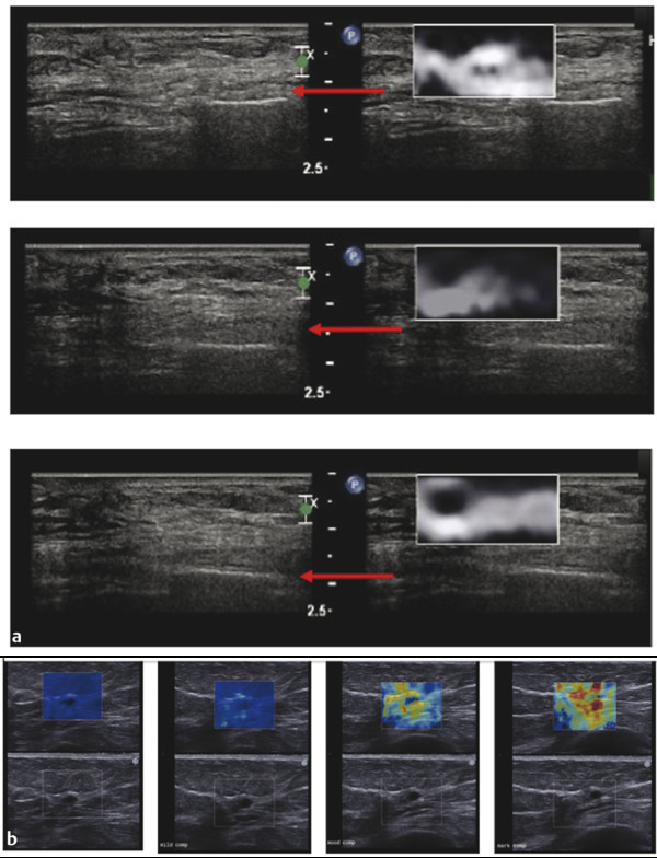
Fig. 2.8 When precompression is applied with the transducer, it can significantly affect both SE and SWE results. In (a), SE images of an epidermoid cyst are presented. The red arrows point to a rib. The upper image has significant precompression, the middle moderate precompression, and the bottom minimal precompression. Note as precompression is released, the rib moves deeper in the image. When minimal compression is applied (bottom image), optimal elastograms are obtained. In this case, the elastograms will be consistent during a cine clip. When moderate precompression is applied, the frames obtained on the release phase are often good; however, those on the compression phase are of poor quality (middle image). When a significant amount of precompression is applied, the elastogram is only noise and is not interpretable (upper image). Similar effects are seen with SWE (b). In this figure, the SWE of a simple cyst is presented with increasing amounts of precompression. The SWSs increase as precompression is applied. Note that rib in the far field is located closer to the transducer as precompression is added. With moderate precompression, a benign lesion can have shear wave speeds (Vs) suggestive of a malignancy.
▶ Fig. 2.9 summarizes the SWS of the different tissue types in the breast at the various amounts of precompression. The amount of precompression is classified into 4 zones: zone A, minimal precompression, 0 to 10%; zone B, mild precompression, 10 to 25%; zone C, moderate precompression, 25 to 40%; and zone D, marked precompression, > 40%.
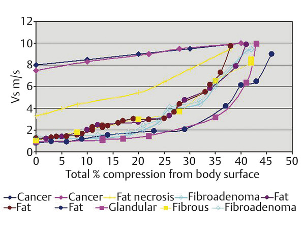
Fig. 2.9 “Average changes in the Vs in tissue types that occur in the breast. We identified 4 regions of precompression that explain clinical elastographic results. In zone A (0%–10% precompression using the technique for measuring precompression), clinical results using both strain and shear wave elastography are not affected. In zone B (10%–25% precompression), strain images with only benign pathologic characteristics begin to degrade, whereas shear wave elastographic measurements increase but in general will not change from a Vs suggestive of a benign lesion to a value suggestive of a malignant lesion. In zones C (25%–40% precompression) and D (>40% precompression), strain images with benign pathologic characteristics show only noise as the elastic properties of all of the tissues become too similar to distinguish. If a malignant lesion is present, strain imaging will be accurate in zones A, B, and C as the elastic properties of normal breast tissues remain different enough from the malignancy to provide accurate results. Benign lesions in zones C and D on shear wave will have Vs and kPa values suggestive of a malignant lesion. It is recommended that all clinical images be obtained in zone A. (Reproduced with permission from Barr RG, Zhang Z. Effects of precompression on elasticity imaging of the breast. J Ultrasound Med 2012; 31:895–902.)
How Can Precompression Affect Strain Elastography Images?
In SE, images are based on the relative stiffness of the lesions within the FOV of an image. It is qualitative (how stiff relative to other tissues in the field of view) but not quantitative (an absolute value). The imaging scale used is relative and based on tissues within the image plane. Using breast as an example, in the case where both soft tissues (fat, fibroglandular tissue) and a very stiff lesion (malignancy) are present in zones A, B, and C, the difference in elasticity (SWS measured in meters per second [m/s]) between the soft tissues and the malignant tissues are adequate to generate an accurate elastogram. However, in zone D the elasticity of both the soft tissues and malignancies are similar; hence, the elastogram is not diagnostic and only represents noise.
However, in a case where the area of interest contains only soft tissues (fat, fibroglandular tissue, soft fibroadenoma, or fibrocystic change) the results are different. In zone A, the elasticity differences between the tissues allows for a diagnostic elastogram. In zone B, the elastogram is borderline for diagnostic value with some frames of good diagnostic quality and some of poor diagnostic value. This is due to precompression, which has made the difference of stiffness between tissues smaller. Based on the author’s experience, this appears to depend on if the frame was taken in a compression or release phase of the cycle. This may be due to the increased precompression on the compression phase of the cycle. In zones C and D, the elasticity properties of the soft tissues are very similar due to the precompression and the elastogram is mostly noise and nondiagnostic.
In one technique to apply a minimal amount of precompression reproducibly,5 a structure in the far field is identified, such as a rib or Cooper’s ligament. The transducer is lifted slowly while watching the structure. As the probe is lifted, the structure will move deeper in the image. While keeping the structure as deep in the image as possible and having adequate probe contact, the elastogram is obtained. The use of ample coupling gel is helpful. This technique has been shown to be highly reproducible both intraoperator and interoperator.5
Another technique that can be used to apply a minimal amount of precompression is to make a standoff pad with coupling gel, making sure some coupling gel is present between the transducer and the patient when obtaining the elastogram.
The quality factor or compression bar used by some vendors does not assess the amount of precompression being applied, just the displacement of tissues during the compression–release cycle. Even when significant precompression is applied leading to a poor elastogram, the quality factor or compression bar can suggest a good elastogram was obtained.
Usually a small amount of precompression (10–20%) is used to obtain B-mode images as it improves B-mode image quality.
2.2.4 Strain Elastography Using ARFI
An ultrasound pulse can be reflected or absorbed (attenuated), or it can transfer its momentum (it can push). This transfer of energy causes tissue to move. Increased energy in the ultrasound beam creates increased force and hence movement. The movement of the tissue has two consequences for elastography: (1) it can be measured directly in strain elastography; or (2) it can generate a lateral transverse (shear) wave through the tissue, the speed of which can be measured in shear wave elastography.
Acoustic radiation force impulse (ARFI),6,7,8 a low-frequency ultrasound pulse which is tailored to optimize the momentum transfer to tissue, can also be used to create the displacement of tissue. The ARFI pulse replaces the patient or probe movement to generate the stress on the tissue. By analyzing the tissue displacement (not the shear waves generated), a SE image can be generated. This technique may be less user dependent than the manual compression technique.
Note that this SE technique is different than SWE technique where the speed of shear waves generated from the ARFI pulse are measured. The SE technique is qualitative (it provides a relative measure of the tissue stiffness in the field of view) while the SWE technique is quantitative (it provides a numerical value of the tissue stiffness). The power of ARFI push pulse is limited by guidelines on the amount of energy that can be put into the body, thus limiting the depth of tissue displacement and therefore the tissue depth of the SE elastogram. This is usually not a problem. When the tissue of interest is too deep, manual displacement technique can be used as it can be adjusted to have appropriate displacement at any tissue depth.
If an ARFI push pulse is used to generate the tissue displacement, no manual displacement (transducer compression-release) should be used. This technique is implemented on one vendor’s system, Virtual Touch Imaging (VTI, Siemens Ultrasound, Mountain View, CA). The probe should be held steady and the patient should refrain from talking, suspend their respiration, and remain motionless during the image acquisition. An ROI box is placed over the area of interest. Because of the power of the ARFI pulse, the system will freeze for a few seconds for transducer cooling. During this period, the system will not respond to knob activation. The color-mapping algorithm is slightly different than that used in the manual compression technique and some differences in the appearance of the elastogram between the two techniques can be seen. In general the ARFI push pulse is limited in producing tissue displacement deeper than 4 to 5cm with most small-parts (e.g., breast, thyroid, testicles, salivary glands) imaging transducers and 8 cm with abdominal transducers. The ARFI pulse is only generated within the ROI box; therefore only the ROI box has strain data within it on the elastogram (▶ Fig. 2.10).
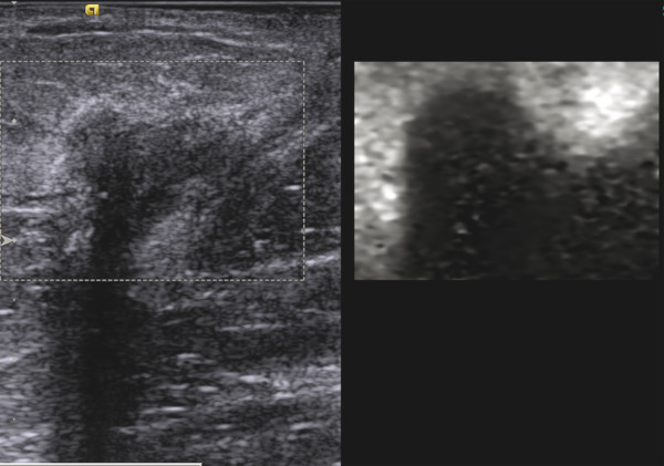
Fig. 2.10 An ARFI pulse creates two types of tissue motion, the displacement of the tissue and the generation of shear waves. When the displacement is tracked, a strain elastogram is obtained. This is an example of an SE elastogram (so only relative stiffness values are displayed) of invasive ductal cancer using Virtual Touch imaging (VTI, Siemens Ultrasound, Mountain View, CA). As opposed to SE using the manual compression technique, the FOV has a maximum allowable size and is placed to include the lesion. Using a very light touch with the transducer on the breast, the patient is asked to remain still and not talk while the update button is pressed to activate the ARFI pulse. The system will freeze for a few seconds and then the VTi image will be displayed. The grayscale map is used here with black as stiff and white as soft. The lesion is significantly stiffer than the surrounding breast tissue.
Related posts:
Stay updated, free articles. Join our Telegram channel

Full access? Get Clinical Tree


