Chapter 13 Quality control
General
The process of measurement, testing or inspection devised to ensure that the function and the performance of a device is achieving a required level is referred to as quality control (QC). The requirement for routine quality control is recognized in the statutory Ionising Regulations (IRMER) [1]. The level required may be set out in Standards agreed by a national or international agency. For example IEC60601 [2], the general standard for medical devices was set by the International Electrotechnical Commission (IEC) which is part of the International Standards Organisation (ISO). IEC60601 was adopted by the European Union and thus became a Standard for the UK. Many parts of this standard concern the safety of radiotherapy treatment machines and simulators and one part particularly relates to the performance requirements and quality control of megavoltage treatment machines [3, 4]. Standards may also be set with respect to what is considered to be good practice or they may be set upon locally based experience. For example, radiotherapy physicists in the UK have identified good practice in many aspects of radiotherapy and published this in a document [5] referred to as IPEM81. An example of a locally set tolerance may be that the field size on a megavoltage treatment machine can be made to lie within ±1.5 mm when another type of machine can achieve ±1 mm for the same amount of work.
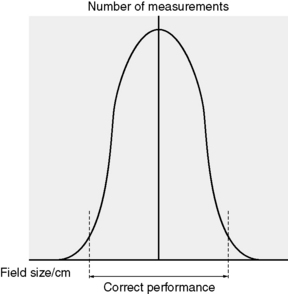
Effective quality control needs to fulfill two roles. One is to demonstrate the correct performance of a system and the other is to detect deterioration of the system in order to take corrective action. Demonstration and detection are, in fact, two sides of the same coin. The boundary between each side is set in accordance with appropriate limits chosen with regard to the distribution of a measured parameter as shown in Figure 13.1 for the example of a 10 × 10 field.
In radiotherapy, quality control has become increasingly significant over the past 20 years. It has been recognized that, in order to achieve and maintain high standards of safe and effective dose delivery, there is a need for not only quality assurance systems which ensure safe, effective and traceable processes, but also for effective quality control checks to demonstrate and ensure satisfactory operation of equipment. In 1985, the ICRP [6] recognized the role that quality control played in the protection of the patient in radiotherapy. The hazards of radiation to normal tissue were well known and the risk of oncogenesis [7–9] further complicates the use of radiation in cancer treatment. These concerns were reinforced by accidents [10], some of which were due to safety failures, others due to performance failures and, of course, some due to human error. It has been clear that the absence or deficiencies of quality control had an adverse affect in some of these accidents. Many accidents highlighted the need for standards to be established in both safety and performance.
The acceptable variation in dose delivery has been identified from clinical experience and radiobiological studies to be ±5% [11, 12]. This gives some perspective on the seriousness of, for example, the Exeter accident in 1988 [13] when a 25% overdose was delivered to many patients between February and July of that year. Systems of quality control checks endeavour to ensure that treatment equipment operates both safely and effectively.
A commitment to quality control
… it is seen that even a person whose treatment had started as early as mid February would not necessarily have shown any abnormal signs until about mid May [13].
An underdose may well go on for a much longer period of time and the incident at Stoke [14], when an underdose of approximately 20% continued for several years, serves as a demonstration of this.
At Exeter, there were clinical concerns by the end of May and the beginning of June 1988. On July 4, the calibration of February 12 was still thought to be correct by the Physics Department and it was not re-measured. No further measurement would have taken place until August. The IPEM dosimetry survey [15] measurement, which revealed the error, was done on July 12.
Frequency, tolerances and failure trends
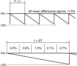
The classical assumption for performance deterioration is a linear change with time. Consider a tolerance of ±3% in dose delivered with action being taken at that level to restore the performance to the required value. Figure 13.2 illustrates such a change in performance with time.
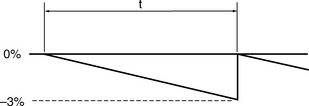
Considering the effect of the length of the time period t:


Hence the length of t can have a variable effect on the dose delivered to the patient.

If t is long, say several times as long as a total course treatment time, T, where typically that can be between 3 to 6 weeks, the following occurs compared to having t equal to T. The variation in the dose is shown in Figure 13.3.
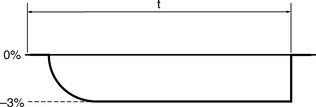
Indeed, the performance deterioration is likely to be far from linear and more likely to be non-linear as in Figure 13.4.
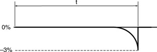
When a parameter is satisfactorily checked and it lies within tolerance it demonstrates compliance. If at the next check the parameter is found to be outside of tolerance then the assumption will be made that it has deteriorated linearly since the previous check. However, the worst case of deterioration will be as in Figure 13.5.
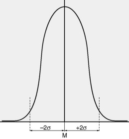
Measurement and uncertainty
Typically, the best estimate is thought of in terms of a Gaussian distribution with a mean, M and standard deviation, σ representing the best estimate and the variation respectively (Figure 13.6).