Quantification of Myocardial Infarction Using a Hidden Markov Random Field Model and the EM Algorithm

Fig. 1.

(left) Typical short axis LGE-MR image where the different types of tissues can be seen within the endocardial (inner) and epicardial (outer) contours. (right) Polar deployment of the LV in the middle image with angle along the vertical axis (myocardium is included between the two contours with LV cavity on the left part)

Several methods have been proposed to estimate the relative part of normal and altered tissues. They can be categorized in 3 types. Threshold based methods evaluate a unique threshold to partition pixels in two classes: pixels belonging to normal myocardium (intensity below the threshold) and pixels associated to necrosis (intensity above the threshold). The most common method evaluates a mean $\mu$ and standard deviation $\sigma$ intensity in a remote myocardial region. The threshold is then defined as $T = \mu + c\sigma$ with c a constant between 2 and 10. The Full Width at Half Maximum evaluates the threshold as half of the highest intensity in the myocardium: $T = I_{max}/2$ . The gaussian mixture model (GMM) defines the threshold as the intersection of two gaussian distributions fitted from the pixel histogram within the myocardium. Classification methods partition the myocardium into several components, basically healthy myocardium, infarct and microvascular obstruction. Fuzzy C-means [3] and support Vector Machine [4] methods have been proposed in this context. Combined methods associate several technics within a workflow. Hsu et al. [5, 6] and Valindria et al. [7] combine threshold based methods and a characteristic analysis to limit false positive. Surprisingly, none of these methods makes use of the local neighborhood and a priori regarding the location of the respective tissue categories. The proposed approach combines a region growing approach within a maximum a posteriori (MAP) optimisation through an Expectation-Maximization (EM) algorithm.

2 Method

Our approach is inspired from the HMRF-EM method by Zhang et al. for the segmentation of brain images [8]. Zhang’s method estimates the parameters of a statistical model from a maximum likelihood estimation with an expectation maximization (EM) algorithm. Let a 2D or 3D image ${\mathbf {y}}= \{y_1, ... ,y_N\}$ and a hidden variable ${\mathbf {x}}= \{x_1, ... ,x_N\}$ , called the label map with N the number of pixels. The endocardial and epicardial contours are supposed to be known as a result from a preliminary manual tracing or (semi)automatic segmentation. In the context of cardiac tissue segmentation, a domain transform is first applied. An initial label map and the corresponding parameters are computed.

2.1 Cartesian to Polar Transformation

We chose to work in polar space for the following reasons (Fig. 1(right)). First, a polar development is well adapted to the LV morphology in short axis views (see Fig. 1(left)). Second, the same weight is attributed to inner and outer pixels/voxels in the polar system while inner layers tend to be underweighted in the Cartesian system. Also, axes for neighboring operations (e.g. morphological) are aligned with the radial and circumferential anatomical directions in the polar system. Last, the 2D image size in Cartesian space is generally $256 \times 256$ while in the transformed polar space, it is around $50 \times 360$ making the processing faster in 2D and 3D. In 3D, this transformation is applied to all the image slices to produce a 3D stack of the unfolded LV myocardium.

2.2 Initial Classification

A first guess for the label map is obtained by extracting the pixel with the most likelihood to belong to the necrosis class. This is obtained with a drastic threshold to keep hyper intense pixels. In practice, we took $T=4I_{max}/5$ with $I_{max}$ the maximum intensity over the whole myocardium. Initial mean and standard deviation for the two zones are computed leading to the initial label map ${\mathbf {x}}^{0}$ and models’ parameters ${\varvec{\Theta }}^{(0)}$ .

2.3 EM Algorithm

The classification problem consists in determining the optimal label map ${\mathbf {x}}^*$ and the statistical model parameters ${\varvec{\Theta }}^{*} = \{\theta _l=(\mu _l, \sigma _l), l \in \mathcal {L}\}$ , with $\mathcal {L}$ being the set of labels given the observed data ${\mathbf {y}}$ . The EM algorithm seeks for a maximum likelihood estimate in two steps. The expectation step computes the expectation of the log likelihood function relatively to the conditional distribution $P(\mathbf x |\mathbf y )$ with the current estimates of the statistical model parameters ${\varvec{\Theta }}^{(t)}$ . 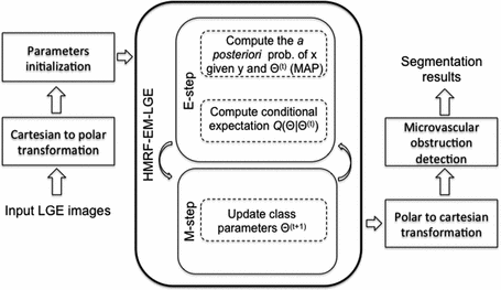The maximization step updates the models’ parameters that maximize the expectation. The whole algorithm is summed up in Fig. 2.

Step E. The E step determines the conditional expectation $Q({\varvec{\Theta }}|{\varvec{\Theta }}^{(t)})$ given by [8]:

$\begin{aligned} Q({\varvec{\Theta }}|{\varvec{\Theta }}^{(t)})= & {} E( \ ln[ \ P({\mathbf {x}},{\mathbf {y}}|{\varvec{\Theta }}) \ ] \ | \ {\mathbf {y}},{\varvec{\Theta }}^{(t)} \ ) \end{aligned}$

(1)

$\begin{aligned}= & {} \sum _{x} P({\mathbf {x}}|{\mathbf {y}},{\varvec{\Theta }}^{(t)}) ln P({\mathbf {x}},{\mathbf {y}}|{\varvec{\Theta }}) \end{aligned}$

(2)

Fig. 2.

Flowchart of the proposed method for the identification of the infarct size and the MVO

According to the Bayes rule, the a posteriori probability of $\mathbf x$ given $\mathbf y$ and ${\varvec{\Theta }}^{(t)}$ reads:

$\begin{aligned} P(\mathbf x |\mathbf y ,{\varvec{\Theta }}^{(t)}) = \frac{P(\mathbf y |\mathbf x ,{\varvec{\Theta }}^{(t)}) P(\mathbf x ,{\varvec{\Theta }}^{(t)})}{P(\mathbf y ,{\varvec{\Theta }}^{(t)})} \end{aligned}$

(3)

Within a Markov Random Field (MRF) framework, both ${\mathbf {x}}$ and ${\mathbf {y}}$ are considered as realization of random fields $X= \{X_i, i \in \mathcal {S}\}$ and $Y = \{Y_i, i \in \mathcal {S}\}$ , respectively ( $\mathcal {S}$ is the set of sites of the MRF, and can be assimilated to pixels here). Using the conventional Gaussian distribution for the probabilities and assuming the conditional independence of sites, the maximization of (3) comes to the minimization of a sum of energies at each site i:

$\begin{aligned} x_{i}^{k+1} = \underset{l \in \mathcal {L}}{argmin}\{ U(y_i|x_i^{k},l) + U(x_{N_i})\} \end{aligned}$