Quantitative Doppler and Hemodynamics
When you can measure what you are speaking about, and express it in numbers, you know something about it; but when you cannot express it in numbers, your knowledge is of a meagre and unsatisfactory kind.
—Lord Kelvin
HEMODYNAMICS IS THE STUDY OF blood flow and its associated forces. The objective of this chapter is to describe the use of Doppler echocardiography for the quantitative assessment of hemodynamics. Although two-dimensional echocardiography displays cardiac dimensions and motion, it does not readily assess cardiac blood flow and pressures. Doppler echocardiography provides excellent assessments of hemodynamics that compare favorably with more invasive measurements. Accordingly, a quantitative Doppler assessment of blood flow, chamber pressures, valvular disease, pulmonary vascular resistance (PVR), ventricular function (systolic and diastolic), and anatomic defects is an essential component of the echocardiographic examination.
The accuracy of the Doppler evaluation depends on the ability to minimize interference from neighboring blood flows and align the ultrasound beam parallel to the blood flow of interest. Traditionally, transthoracic echocardiography was a superior approach because it offered multiple windows and angles from which blood flow could be interrogated. The introduction of multiplane transesophageal echocardiography (TEE) has increased the number of imaging windows and angles from which the heart can be evaluated with TEE and has greatly facilitated accurate hemodynamic evaluation.
VOLUMETRIC BLOOD FLOW CALCULATIONS
Doppler Measurements of Stroke Volume and Cardiac Output
Principles
In many instances, knowledge of the volume of blood flow is desired. Cardiac output (CO) and stroke volume (SV) are familiar examples. It is important not to confuse blood flow velocity, which is the speed at which blood flows (expressed in centimeters per second), with volumetric flow, which is the amount of blood that flows (expressed in cubic centimeters per second). The volumetric flow (Q) at any point in time equals the blood flow velocity (v) times the cross-sectional area (CSA) of the conduit.
Q = v × CSA
To determine the volumetric flow with echocardiography, a Doppler measurement of the instantaneous blood flow velocities and a two-dimensional measurement of the CSA are required.
In the clinical setting, the volume of blood produced during each cardiac cycle, known as the SV, is an important parameter of cardiac performance. To calculate the SV, the instantaneous velocities during systole are traced from the spectral display, and the internal software package of the echocardiographic system calculates the time–velocity integral (TVI), which is expressed in centimeters (Fig. 6.1). Conceptually, the TVI represents the cumulative distance, commonly referred to as the stroke distance, that the red cells have traveled during the systolic ejection phase. When the stroke distance is multiplied by the CSA (in square centimeters) of the conduit (e.g., aorta, mitral valve [MV], pulmonary artery [PA]) through which the blood has traveled, the SV (in cubic centimeters) is obtained (1–7). CO, which expresses volumetric flow in cubic centimeters per minute, is estimated from the product of the SV and the heart rate (HR).
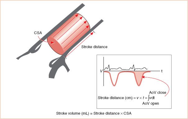
FIGURE 6.1 Determination of stroke volume. Volumetric flow can be determined from a combination of area and velocity measurements. In this example, flow through the ascending aorta is used to determine the stroke volume. Integrating the Doppler-derived flow velocities over time (known as the time–velocity integral) during a single cardiac cycle calculates the stroke distance. The cross-sectional area measurement is obtained with two-dimensional echocardiography. The product of these two measurements, conceptualized as a cylinder, is the stroke volume. CSA, cross-sectional area; AoV, aortic valve.
Echocardiographic Technique for Doppler Measurements of Stroke Volume
The SV and CO are best measured with TEE at the left ventricular outflow tract (LVOT) or aortic valve (AoV) (1–7). These locations offer several advantages to the clinical echocardiographer. First, the entire ejected SV traverses these structures, whereas it does not in more distant vessels, so that the total SV can be calculated. Second, Doppler interrogation typically assesses blood flow from only a small fraction of the total CSA of the vessel, and therefore SV calculations assume that the measured velocity reflects the mean flow velocity throughout the cross section of the vessel. This assumption is most accurate when blood flow is laminar and has the same velocity across the entire vessel, a situation known as a blunt or flat flow profile (Fig. 6.2). Since the blood is accelerated along the truncated LVOT during systole, the velocity profile has a blunt, uniform pattern rather than the parabolic pattern seen in the ascending aorta or PA. Consequently, the LVOT and AoV are attractive because the risk for sampling blood velocities that are not reflective of the average blood flow velocity is reduced. Third, the LVOT and ascending aorta are more circular and the CSA changes less during the cardiac cycle. Multiplane TEE offers excellent windows at these sites for both Doppler blood flow measurements and two-dimensional echocardiographic measurements of the CSA. Several clinical studies have confirmed that the CO measurements obtained by TEE compare favorably with those obtained by thermodilution (1–3,5–7).
LVOT or transaortic valvular flows are most reliably obtained from the transgastric (TG) long-axis and the deep TG long-axis views because the blood flow is nearly parallel to the ultrasound beam. It is critical to interrogate blood flow carefully through minor alterations in the probe position and multiplane angle to obtain the optimal Doppler spectral signal. The maximal velocity profile with a dense spectral signal is sought.
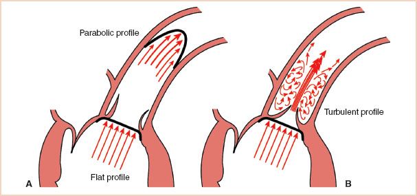
FIGURE 6.2 Common flow profiles. A: The acceleration of the blood flow as it enters the truncated left ventricular outflow tract leads to a “flat” profile in which velocities are uniform. As blood travels in the ascending aorta, the effects of wall friction and a curved conduit result in an asymmetric and parabolic flow profile. B: When blood is forced through a narrow opening, laminar flow is replaced with turbulence. In this illustration, aortic stenosis has created a narrow, high-velocity jet encased by turbulent flow.
Calculation of the left Ventricular Outflow tract Stroke Volume
1. The pulsed wave Doppler sample volume is positioned in the LVOT immediately proximal to the AoV (TG long-axis and deep TG long-axis views).
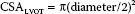
2. The CSA for the LVOT is best obtained from the midesophageal (ME) LVOT view. The CSA is calculated from a measurement of the LVOT diameter as follows:
Calculation of the Transaortic Valve Stroke Volume
1. The continuous wave Doppler beam is directed through the AoV orifice from the TG long-axis or deep TG long-axis view (Fig. 6.3).
2. The CSA of the valve is best estimated by planimetry of the equilateral triangle-shaped orifice observed in midsystole (6). The AoV is viewed in cross section from the ME AoV short-axis window, and frame-by-frame review is used to capture the valve in midsystole. Planimetry of the triangle-shaped orifice yields the effective CSA.
Calculation of the Stroke Volume of the Right Side of the Heart
Alternatively, right-sided flows and diameters can be analyzed from the main PA or the MV. Pulsed wave or continuous wave Doppler analysis proceeds after the main PA is imaged from high esophageal windows at the level of the superior mediastinal vessels (Fig. 6.4) or the right ventricular outflow tract (RVOT) is imaged from TG windows at 110- to 150-degree rotation of the transducer and rightward turn of the TEE probe (Fig. 6.5). In all cases, the maximal velocity profile is sought. Flow across the MV is measured by placing the sample volume at the level of the mitral annulus to obtain the transmitral TVI, which is then multiplied by the area of the MV annulus. Compared with the diameters of the LVOT and ascending aorta, the diameters of the main PA and MV fluctuate more during the cardiac cycle, and these measurements are less reliable than those from the LVOT and AoV (4). In addition, the MV orifice is not circular, and its size changes during diastole.
FIGURE 6.3 Stroke volume (SV) calculated from the left ventricular outflow tract (LVOT). The right panel demonstrates measurement of the left ventricular outflow tract (LVOT) diameter (2.2 cm) from the midesophageal long-axis window. The left panel shows pulse wave (PW) Doppler measurement of blood flow velocities across the LVOT (TVILVOT) from the deep transgastric left ventricular outflow tract window. The time–velocity integral (TVILVOT) is 16 cm. The cross-sectional area of the LVOT (CSALVOT) is calculated from the measured diameter using the equation: π(D/2)2. The calculated area of the LVOT (3.75 cm2) multiplied by the TVI (16 cm) yields a stroke volume of 60 mL/beat. When multiplied by the heart rate (HR), the cardiac output is obtained.
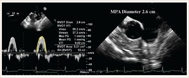
FIGURE 6.4 Calculation of cardiac output from the main pulmonary artery (MPA) performed from the ME ascending aortic SAX view seen in the right panel from which the MPA diameter (2.6 cm) can be measured. The MPA time–velocity integral (TVI) is assessed by the pulsed wave Doppler beam being aligned with pulmonary artery blood flow and with the sample volume placed at the same location (plane) where the MPA diameter was measured. The cross-sectional area (CSA) of the pulmonary artery (π[D/2]2) is calculated as 5.3 cm2. Manual tracing of the spectral display of pulmonary blood velocities shows a TVI of 9.92 cm. When multiplied by the CSA, the stroke volume is calculated as 53 mL/beat. Diam, diameter; SV, stroke volume.
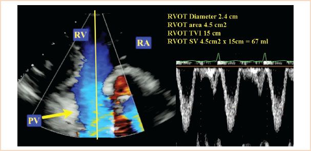
FIGURE 6.5 Stroke volume (SV) through the right ventricular outflow tract (RVOT) was calculated from the transgastric right ventricular inflow/outflow window. The product of the RVOT area (4.5 cm2) and the RVOT time–velocity integral (TVI; 15 cm) was used with RVOT area calculated from the RVOT diameter measurement (2.2 cm; area = π[D/2]2). PV, pulmonary valve; RA, right atrium; RV, right ventricle; TVI, time–velocity integral; D, diameter.
Regurgitant Volume
Regurgitant volume is the quantity of blood that flows back through a regurgitant lesion in a single cardiac cycle. The total SV traversing a regurgitant valve during systole is greater than that in a normal valve. For a regurgitant valve, the total SV equals the regurgitant volume plus the SV delivered to the peripheral circulation. The regurgitant volume can be calculated as the difference between the total forward flow through the regurgitant valve and the total forward flow through a reference valve.
Regurgitant volume = forward flow through regurgitant valve – forward flow through reference valve
In the case of mitral regurgitation (MR) (in the absence of significant AoV disease), the SV across the AoV can be used as the true SV.

However, there is a significant potential for error in the mitral flow measurements because the MV orifice is not circular (4), and its diameter changes during the cardiac cycle.
Similarly, the aortic regurgitant volume can be calculated as follows:
Regurgitant volumeAV = forward flow through AoV – flow through MV
The regurgitant fraction is simply the ratio of the regurgitant volume to the total SV through the diseased valve and is typically expressed as a percentage:
Regurgitant fraction (%) = regurgitant volume/forward flow
Alternative techniques to measure the severity of valvular regurgitation are discussed in Chapters 8 and 11.
Intracardiac Shunts
The ratio of pulmonic to systemic SV, Qp/Qs, is important in assessing the severity of shunts and in guiding treatment. Intracardiac shunts are assessed by calculating the SV (8). By measuring the left-sided (LVOT or AoV) and right-sided (PA or RVOT) SVs, one can determine Qp/Qs:

These measurements are often combined with two-dimensional and color Doppler data to provide a complete assessment of congenital lesions.
Valve Area: The Continuity Equation
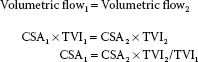
The principle of conservation of mass is the basis of the continuity equation, which is commonly used to measure the AoV area (9) (Fig. 6.6B). The continuity equation simply states that the volume of blood passing through one site (e.g., the LVOT) is equal to the mass or volume of blood passing through another site (e.g., the AoV). Of course, there must be no intervening channels for this principle to apply. By using the principle of volumetric flow, discussed earlier, the continuity equation can be applied clinically.

FIGURE 6.6 Calculating the pressure gradient and valve area. A: Bernoulli equation. The simplified Bernoulli equation states that the pressure drop (P2 − P1 = Δ 4P) across a stenotic orifice is four times the square of the velocity of the high-velocity jet. P1, blood pressure proximal to stenosis; v1, flow velocity proximal to stenosis; P2, blood pressure distal to stenosis; v2, flow velocity through stenosis. B: Continuity equation. The continuity equation is often described as the principle of “what goes in must come out.” Accordingly, flow proximal to the stenosis (A1 × v1) should equal flow through the stenosis (A2 × v2). A1, cross-sectional area proximal to stenosis; v1, flow velocity proximal to stenosis; A2, cross-sectional area of stenosis; v2, flow velocity through stenosis.
To calculate the area of the aortic valve (AoV):
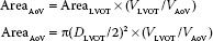
where DLVOT is the diameter of the LVOT and VLVOT is the velocity in the LVOT.
TEE assessments of LVOT and aortic flows and LVOT diameter were described earlier in the section “Doppler Measurements of Stroke Volume and Cardiac Output.” The continuity equation is the basis for assessments based on the proximal isovelocity surface area method (10–12), which is described in detail in Chapter 9.
INTRACARDIAC PRESSURES AND PRESSURE GRADIENTS: THE BERNOULLI EQUATION
Pressure gradients are used to estimate intracavitary pressures and to assess conditions such as valvular disease (e.g., aortic stenosis), septal defects, outflow tract abnormalities (e.g., LVOT obstruction), and major vessel pathology (e.g., coarctation). As blood flows across a narrowed or stenotic orifice, blood flow velocity increases. The increase in velocity is related to the degree of narrowing. The Bernoulli equation describes the relation between the increases in blood flow velocity and the pressure gradient across the narrowed orifice (13):
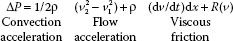
where P is the pressure gradient across the area of interest (mm Hg), ρ is the density of blood (1.06 × 10³ kg/m3), v1 is the peak velocity of blood flow proximal to the area of interest (m/s), and v2 is the peak velocity of blood flow across the area of interest (m/s).
In clinical practice, the Bernoulli equation is simplified by ignoring the effects of flow acceleration, viscous friction, and the velocity proximal to the area of interest (v1) because of the following:
1. Peak flows are of interest in clinical measurements. During peak flow, the flow acceleration is virtually nonexistent and thus can be ignored.
2. Viscous friction contributes significantly only in discrete orifices with an area of less than 0.25 cm2. Blood flow is thought to be constant for orifices with an area greater than this, so that viscous friction is also eliminated in the Bernoulli calculation.
3. For clinically significant lesions, v2 is substantially greater than v1, such that v22 − v12 is approximated by just v22.
The elimination of these factors yields the simplified Bernoulli equation:

Therefore, a pressure gradient is obtained in clinical echocardiography by the straightforward process of measuring the peak velocity of blood flow across the lesion of interest (Fig. 6.6A). However, when v1 is greater than 1.4 m/s then the Modified Bernoulli equation is considered to account for the higher proximal velocity:

To calculate the pressure gradient, the pulsed wave Doppler sample volume or continuous wave Doppler beam is directed across the region of interest. The measured peak velocity is then entered into the simplified Bernoulli equation (ΔP = 4v22) to estimate the pressure gradient. When blood flow velocities are high (≥1.4 m/s), continuous wave Doppler is preferred to avoid the aliasing that may occur with pulsed wave Doppler. It is imperative that the Doppler beam be positioned so that it interrogates the jet with the highest velocity; otherwise, the pressure gradient will be significantly underestimated. To obtain the highest velocity flow, interrogation from multiple windows is preferred. Also, accuracy is improved by assessing multiple flow profiles (3 to 5 for a regular rhythm and 10 for an irregular rhythm) at end-expiration. The simplified Bernoulli equation is the basis for most pressure gradient calculations in clinical echocardiography.
Assessment of Valvular Disease
The Bernoulli equation is most commonly used to measure the pressure gradient across a stenotic valve. This application is illustrated in Figure 6.6A. The assessment of valvular stenosis is discussed extensively in Chapters 9 and 12.
In addition, the rate of decline in the pressure gradient across the valve is related to the severity of disease (14). The pressure half-time is the time required for the peak transvalvular pressure gradient to decrease by 50%. Typically, a larger orifice has a shorter pressure half-time because pressure can equalize more quickly. The assessment of mitral stenosis and aortic insufficiency (AI) can be aided by pressure half-time measurements (see Chapters 9 and 12).
Measurement of Intracavitary Pressures
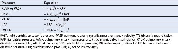
Intracavitary and pulmonary arterial pressures can be measured by combining a Doppler-derived pressure gradient from a regurgitant jet and a known (or estimated) pressure either proximal or distal to the chamber of interest (Table 6.1). Since accuracy depends on alignment of the ultrasound beam with the blood flow, velocities of central regurgitant jets are more accurately assessed than those of eccentric jets.
Right Ventricular Systolic Pressure and Pulmonary Artery Systolic Pressure
With the simplified Bernoulli equation, the peak velocity of the tricuspid regurgitant (TR) jet is used to calculate the pressure gradient between the right ventricle (RV) and right atrium (RA) (15). The peak TR velocity is obtained by placing the continuous wave Doppler beam parallel to the regurgitant jet. By adding a known or estimated right atrial pressure (RAP) or central venous pressure (CVP) to the RV–RA pressure gradient, the right ventricular systolic pressure (RVSP) is estimated. In patients without significant pulmonic valve stenosis or RVOT obstruction, the RVSP and pulmonary artery systolic pressure (PASP) are similar (Figs. 6.7 and Figs. 6.8).
TABLE 6.1 Calculation of Cardiopulmonary Pressures
Related posts:
 A Practical Approach to the Echocardiographic Evaluation of Ventricular Diastolic Function
 Prosthetic Valves
Stay updated, free articles. Join our Telegram channel

Full access? Get Clinical Tree


