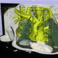
Fig. 5.1
Three-dimensional visualization used by neurosurgeons to examine the relationship of pathology to familiar landmarks. These visualizations are used for preoperative surgical planning as well as intraoperative guidance and verification [1]
The focus of this chapter is on segmentation and registration in image-guided therapy. In practice, the tasks of registration and segmentation are complementary and are inextricably linked. Registration is facilitated by segmented images and is not possible without basic segmentation in the form of pixel labeling or image intensities. Likewise, segmentation is facilitated by registration to other images, e.g., an atlas with expert segmentation labels [2], in which complementary information can be used to drive segmentation. This chapter aims to provide an overview of segmentation and registration individually, in the context of image-guided therapy, including fundamental methods and validation techniques. Joint investigations of segmentation and registration are not explicitly discussed; however, the interested reader is referred to the literature [3].
Registration
Image-guided therapy involves acquiring images of a patient using different modalities at different points in time, from pre-procedural diagnosis and planning, to intra-procedural guidance and visualization, and finally to post-procedural assessment. The goal of registration is to align different images of the same underlying tissue or patient into a common reference frame, for the purpose of visualization and navigational guidance over the course of therapy.
Registration can be accomplished by a variety of means. Manual registration can be performed, where a human manipulates images via a software interface. Registration can be performed visually; for instance, in the context of neurosurgery, the surgeon can mentally fuse intraoperatively acquired ultrasound (US) with a magnetic resonance (MR) volume acquired preoperatively and used in surgical planning, in order to carry out the procedure. Tracking devices external to the image can be used, again in the context of neurosurgery; the 3D position and orientation of the US probe can be determined by a stereo camera system in the context of a neuronavigation system and related to the preoperative MR via a 3D rigid transform for display.
Automatic image registration involves the use of computational algorithms to establish image alignment based on image intensity data. A large body of research literature has been dedicated to the study of automatic image registration. This section aims to highlight general considerations and techniques that apply to the context of image-guided therapy and to describe several concrete examples.
General Approach
Automatic registration aims to align images into a common coordinate system or reference frame. Here we assume that there are two images to be registered, where one image is chosen as a fixed image or model I and the other is considered a moving image J, and the goal of registration is to identify a spatial transform T mapping locations in J to I. Registration is driven by a measure of image similarity that quantifies the degree to which image intensities in I and J agree, given a mapping T. In general, T is non-unique in the sense that there may be many mappings that are equivalent in terms of image similarity. Furthermore, registration must typically process large amounts of image data, and it is generally intractable to consider all possible mappings between images. Additional constraints are thus placed on permissible mappings T, in order to bias registration towards solutions that agree with prior expectations and to reduce computational complexity.
Transformation Model
The transform model determines the space of permissible spatial mappings T between I and J and should be chosen to reflect the true underlying mapping as closely as possible. The general context of image-guided therapy typically involves intra-subject registration, e.g., where the images to be aligned are acquired from the same physical tissue, and T can thus be designed to follow a physically justified model mapping tissues from one image to the next. Furthermore, in a number of contexts, tissue may be present in one image but absent in another, for instance, due to surgical resection and the introduction of instruments. In such contexts it is important to model the event that a valid mapping may not exist in certain regions of the image.
In the case where little shape change has occurred between image acquisitions, a low-parameter linear transform model, e.g., a rigid transform, is sufficient, for example, images of the head prior to major resection in an image-guided neurosurgical context. In general, however, soft tissues tend to deform over the course of a therapeutic procedure, and nonlinear transform models may be required. A biomechanical tissue model can be used, that takes into account the physical properties of the underlying tissue. For example, the image can be represented by a finite element model (FEM) consisting of a mesh where interactions of mesh nodes are governed by physical properties such as elasticity [4, 5]. The FEM can be modified to account for physical phenomena such as gravity and resection [6]. Tissue properties may be difficult to specify in a biomechanical model, and various classes of alternative nonlinear transforms can be used, for example, deformation fields governed by splines [7] or local translations [8] (Fig. 5.2).
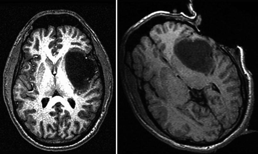

Fig. 5.2
Preoperative (left) and intraoperative (right) MR images of a brain with a tumor. The transform model might include global rotation, nonlinear deformation in the neighborhood of the tumor, and occlusion in the area of resection
Patient Motion: Tissue deformation caused by patient motion is a confounding factor. Motion due to respiration is important in abdomen and thoracic procedures; this can be reduced via breath holding or accounted for by maintaining a temporal model accounting for tissue movement over the breathing cycle [9]. Cardiac motion during can be accounted for by acquiring and registering pre- and intra-procedural images at the same point in the cardiac cycle [10].
2D–3D: Registration may be important in cases where image intensities are sampled in different image dimensions. Modalities such as computed tomography (CT) and MR sample volumetric data in three spatial dimensions; however, other technologies such as X-ray, fluoroscopy, or B-mode US sample in two spatial dimensions. To register images of different spatial dimensionality, the transform must account for the image formation model, for instance, projection and attenuation in X-ray or fluoroscopy [1]. In the case of a 2D projection based imaging modality such as X-ray, registration typically attempts to determine a rigid transform, for example in case of registration between 2D intra-procedural fluoroscopic and pre-procedural 3D CT cardiac images [10], 2D pre-procedural portal and pre-procedural 3D CT cardiac for patient positioning in the context of radiation therapy [11]. In the case of 2D US data, the image represents a slice through a 3D volume, and a navigation system is typically used to track the position of the US probe and slice plane relative to the 3D volume. Registration can then be accomplished by either aligning 2D slice data directly with the 3D volume [12], or by creating a 3D US volumetric image from US slices and performing 3D-3D registration [13].
Occlusion: Registration in the context of image-guided therapy must often consider the scenario where tissue or objects may be occluded, or not present in all images being registered. For example, tissue may not be present in all images due to resection, may not be recognizable or visible due to properties of different image modalities, or the images may contain instruments.
The issue of occlusion scenario raises a challenge for registration, in that there may be regions in which a valid image-to-image mapping may not exist. Registration techniques may be unaffected by minor occlusions and produce reasonable results [14]; however, in significant occlusion, it is important to address the issue directly. An occlusion model can be explicitly incorporated, delineating image regions of anomalous image intensity where T may be undefined over the course of registration [15]. Registration can focus on identifying local image regions where correspondence is most probable, local block matching strategies register local regions independently throughout the image, and then identifying a transform supported by the majority of regions [8]. Informative image regions can be identified by saliency operators and used to improve registration [12].
In the case of therapeutic planning, prior information may be available as to how the images may be affected during the course of the procedure, for instance, regions in which resection may occur and the location and appearance instruments. Such information can be incorporated into the registration process in order to more effectively model occlusion, for instance, resection and retraction of brain tissue in the case of neurosurgery [6, 16].
Image Similarity
Registration is driven by a measure of image similarity, given a transform T. For effective image similarity measurement, the images being registered must exhibit contrast from homologous structures. Similarity may be computed between image intensity data or between measurements or features derived from intensity data such as hierarchical features [17], probabilistic intensity class labels [12], combined intensity, and gradient information [18]. In data defined purely by geometrical features, e.g., points or surfaces derived from anatomical structure in images, individual features bear no distinguishing information. Similarity is thus evaluated based on the geometry of feature sets, e.g., the sum of nearest-neighbor distances (i.e., the Procrustes measure) [19].
In the general case where data consists of intensity measurements, similarity measures can be generally understood by the assumptions made regarding the joint relationship between data [20]. Measures such as the sum of squared differences (SSD) or correlation assume a linear relationship between data and are useful and computationally efficient in the case of intra-modality registration. The correlation ratio [21] assumes a functional relationship between data and can be used where data exhibit nonlinear contrast differences. The mutual information (MI) [22] and normalized mutual information (NMI) [23] assume only a statistical relationship between data and can be used in the general case of multimodal image alignment. MI is powerful but computationally intensive, and in general the joint relationship between image data can be learned from training images [24], after which point similarity can be computed via maximum likelihood methods. Figure 5.3 illustrates the joint relationship between corresponding intensity measurements in proton density (PD) and MR images; note the nonlinear nature of the relationship between intensities.
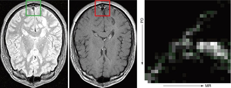

Fig. 5.3
The left and center images are proton density (PD) and T1 MR images of a brain; squares indicate regions of interest (ROIs). The rightmost image shows the joint intensity histogram (right) generated from corresponding intensity samples within the ROIs
Optimization
Image registration typically involves identifying a value of T that maximizes or optimizes a fitness function f(I,J,T) including terms for image similarity and the transform model. A variety of optimization methods can be brought to bear in this respect, depending on the formulation of f(I,J,T), and generally described as global or local in nature. Global optimization identifies the transform T that results in the extremum of f(I,J,T). Such optimization is typically only feasible for transform models consisting of a small number of parameters, for instance, image translations, for which an exhaustive search can be performed over the range of possible T. Such a global search is generally computationally prohibitive, and instead local optimization methods are typically used. Local optimization operates on the principle that f(I,J,T) is a smooth function of T, and that a path can be followed starting from an initial transform to a local maximum in an iterative fashion. A number of local optimization techniques exist [25]. Gradient ascent strategies such as Newton’s method or the conjugate gradient method iteratively update T according to the gradient of f(I,J,T) until a maximum is reached. The simplex method and Powell’s method modify T without requiring gradient computation and may be useful in cases where the gradient of f(I,J,T) may be difficult to calculate. The expectation maximization (EM) algorithm [26] is used in a maximum likelihood framework, iteratively computing expected values of registration parameters, then updating their likelihoods.
Local optimization techniques are prone to converging to suboptimal local maxima, and a variety of methods have been proposed to avoid this difficulty. Simulated annealing or genetic algorithms randomly perturb the solution during a search and are helpful in avoiding suboptimal local maxima. Coarse-to-fine or multi-resolution [27] optimization strategies operate by first computing registration of large-scale image structure at low image resolution, then using these results to guide finer-scale alignment at higher image resolutions. Multi-resolution optimization is useful in both speeding up registration and avoiding suboptimal minima.
Validation
Validation of registration methods is an important consideration; here we focus validation of automatic registration in terms of accuracy, precision, and robustness. Various other validation considerations exist; Maintz et al. [28] list resource requirements, algorithm complexity, assumption verification, and suitability for clinical use. These considerations may vary from one clinical context to the next, and we refer the reader to [28] for further reading.
In the context of image-guided therapy, it is important to know the accuracy and precision with which registration is capable of correctly aligning or localizing therapeutic targets, for instance, a tumor in image-guided radiation therapy or surgery. Accuracy is typically evaluated retrospectively by comparing the mapping T obtained by registration against ground truth. Ground truth can consist of locations of fiducial points, surfaces, or regions defined manually or automatically in the images registered.
The accuracy of ground truth regions is typically evaluated by measures of overlap, for instance, the Jaccard index [29] or Dice’s coefficient [30], also used in image segmentation. The Jaccard and Dice measures are useful in that they measure registration accuracy in a manner independent of the number of image measurements or voxels. The drawback of overlap measures is that, while they quantify the ability of registration to align homogenous regions, they do not effectively quantify the accuracy of the spatial mapping. For instance, perfect overlap can generally be achieved by multiple, possibly physically implausible spatially mappings between ground truth regions.
The accuracy of ground truth can be defined in terms of image boundaries or surfaces in the image, for instance, where the goal is to correctly register tumor margins in preoperative and intraoperative surgical images [31]. The Hausdorff distance [32] measures the maximum discrepancy between two point sets and can be used to evaluate the agreement between registered boundaries. For the same non-uniqueness line of reasoning with overlap measures, boundary-based discrepancy measures do not necessarily reflect the correctness of the registration mapping T.
Validation of registration accuracy has been perhaps most studied in the context of quantifying the discrepancy between ground truth point landmarks or fiducials. Unlike region or boundary labels, fiducial points make it possible to estimate the accuracy of the spatial mapping T directly. The quantities of interest in quantifying accuracy are the fiducial localization error (FLE) and fiducial registration error (FRE) [33]. FLE is the intrinsic error in localizing of fiducial landmarks in a single image, e.g., markers or distinctive anatomical structures, and the FRE is the error in landmark alignment following registration. In certain cases fiducial landmarks associated directly with the target of interest are not available, e.g., a low-contrast tumor; in these cases the target registration error (TRE) can be estimated as a function of the FRE. The case of point-to-point rigid registration has been intensely studied [33, 34]; nonrigid registration accuracy is also quantified in terms of fiducial landmark error [35].
While registration accuracy has been addressed in a relatively large body of literature, other important validation considerations include precision and robustness, which have been less studied. Precision refers to the repeatability with which registration obtains the same results across similar conditions. Precision is difficult to calculate directly, but estimates can be obtained via sampling techniques, for instance, performing registration trials by artificially deforming intensities in one image and inspecting the covariance of results [2]. Robustness refers to the ability of registration to converge to a reasonable result despite the presence of outliers or incorrect initialization. The literature contains few measures of robustness; in general the “capture radius” is often cited [36], i.e., the range of deviation about the true mapping within which optimization can converge to a correct solution.
Segmentation
Segmentation of digital medical imagery is a labeling problem in which the goal is to assign to each voxel in an input gray-level image, a unique label that represents an anatomical structure. This labeled image is referred to as the “segmentation” of the input image or the “segmented” image. An example input grayscale image is a magnetic resonance imaging (MRI) scan of a human head in Fig. 5.4. A labeling or segmentation for one such cross-sectional image into skin, brain tissue, ventricles, and tumor, and three-dimensional visualizations created from such segmentations of a complete scan are shown in Fig. 5.5.
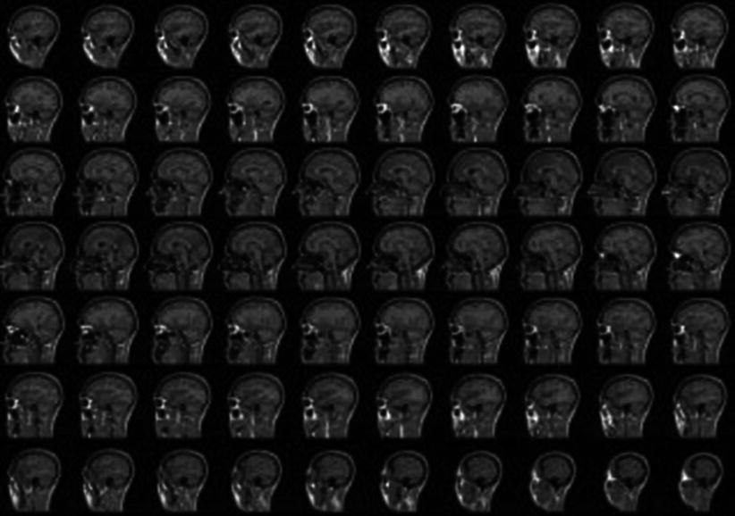
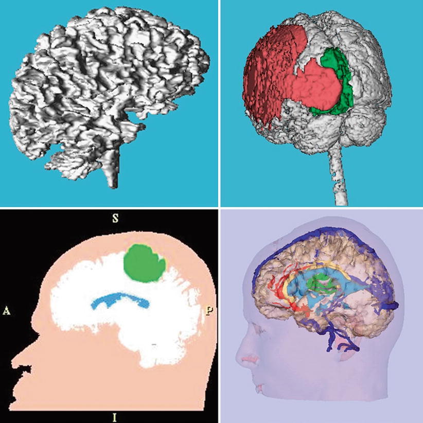

Fig. 5.4
A set of two-dimensional sagittal cross-sectional slices comprising a 3D brain MRI scan. This is the view of an MRI scan that is printed on film and mounted on a light-box and is traditionally available to clinicians to aid them in making diagnosis and in planning therapy

Fig. 5.5
Top row left: a 3D rendering for visualization of the white matter from an MRI scan of a normal subject. Right: a three-dimensional rendering of the brain surface of a patient, overlaid with pathology which is shown in green and red. Bottom left: a segmented MRI slice showing skin in pink, brain tissue in white, ventricles in blue, and tumor in green. Right: a three-dimensional rendering of segmented skin surface, brain tissue, major blood vessels, and tumor from a diagnostic MRI scan
Segmentation Nomenclature
Based on the nature of the inputs required and outputs generated by a segmentation method, it may be categorized into one or more of the following classes.
Binary or Multilabel: If the number of output labels in segmented images is 2 or greater than 2.
Supervised vs. Unsupervised: If a set of labeled images or “training data” is available to the segmentation method to “learn” the differences between the underlying classes, the method is considered supervised, vs an unsupervised method which deduces the characteristics of the classes without training data.
Hard vs. Soft Segmentation: A hard segmentation method is one in which the output of the segmentation is a unique label at each location in the image. A soft segmentation method is one in which the output is the probability of each class at each location in the image.
Intensity–Based vs. Model–Based Segmentation: Purely intensity-based segmentation methods, also referred to as classification methods, assign labels based solely on gray-level values in the image. Model-based methods combine the image gray levels with explicit or implicit models of the underlying structures that are to be segmented.
In sections “Graph Based Segmentation, Particle Filters, and Interactive Segmentation” we summarize approaches to segmentation that have gained momentum in the last decade and that we believe will continue to be applied to image-guided therapy (As mentioned earlier in this chapter, joint investigations of segmentation and registration are a very interesting development of the last decade as well, and we refer the interested reader to our other recent publications on that topic [3]). And in sections “Braintumor: Glioma Segmentation and Segmentation for Prostate Interventions” we then describe how image segmentation has been used specifically to guide neurosurgery and prostate interventions.
Graph-Based Segmentation
The formulation of image segmentation as a graph-partitioning problem was introduced in [37] and in our view has been an influential approach that has led to several successful developments in the last decade [38–40].
In a graph representation, each pixel in the image is a node in the graph, and a subset of neighboring pixels is connected by edges. Weights on the edges measure how dissimilar the nodes are. Graph-based segmentation methods partition an image by selecting a subset of these edges from the graph. While graph-based segmentation methods were developed successfully in the last decade, the underlying theory traces back to Markov Random Fields which had previously been used as a basis for image representation and segmentation. Solving MRFs is an NP-hard problem and is typically accomplished via iterative algorithms. However, using a graph representation, globally optimal segmentations can be obtained in polynomial time by solving the maxcut/minflow problem using the Ford-Fulkerson algorithm [41]. Notable extensions in the last decade include solving the graph cut in N-dimensions [42], an iterative and interactive approach where the edges are re-weighted according user input [43], and a formulation that restricts the graph cut by using additional user-defined seed points to set up fixed nodes in the graph [44, 45].
Particle Filters
Another category of image segmentation in the field of computer vision is tracking moving and deforming objects. A typical current example is the automatic tracking of persons in a security camera video stream. In medical image processing, the lung is a moving and deforming organ that makes automatic delineation over time a challenging task. Tracking the lung is especially relevant in image-guided radiation therapy, where modeling complex tumor motion is important in order to achieve optimal dose delivery and to avoid or minimize radiation of the surrounding healthy tissue. In contrast to static images for segmentation and registration problems, tracking involves estimating the global motion of the object and its local deformations as a function of time. Particle filters – also known as sequential Monte Carlo methods – use swarms of points (so-called particles) to approximate posterior densities. This approximation is realized by assigning a weight to each particle and uses a discrete distribution of the particles which results in particle probabilities that are proportional to the particle weights [46]. Particle filters were introduced by Gordon et al. in 1993 in order to implement recursive Bayesian filters [47]. Since then, several algorithms based on this original approach have been developed that differ primarily in the way particle swarms evolve and adapt to input data [48]. For example, Rathi et al. [49] formulate a particle filtering algorithm in the geometric active contour framework that can be used for tracking moving and deforming objects. They propose a scheme which combines the advantages of particle filtering and geometric active contours realized via level set models for dynamic tracking. A probabilistic algorithm for simultaneously estimating the pose of a mobile robot and the positions of nearby people in a previously mapped environment called the conditional particle filter was introduced by Montemerlo [50]. The method tracks a large distribution of people locations conditioned upon a smaller distribution of robot poses over time.
Stay updated, free articles. Join our Telegram channel

Full access? Get Clinical Tree


