Fig. 10.1
(a) Schematic drawing of the arterial supply and venous drainage of the kidneys. CT celiac trunk, CIA common iliac artery, CIV common iliac vein, LGV left gonadal vein, LSRV left suprarenal vein, PHA proper hepatic artery, RA renal artery, RGV right gonadal vein, RSRV right suprarenal vein, SMA superior mesenteric artery. (b) Schematic drawing of the renal arteries. AIL interlobar artery, AILL interlobular artery, AR renal artery, AS segmental artery. (Drawing by Blankvisual, Thun, Switzerland)
The renal arteries give rise to five segmental arteries (Fig. 10.1b). The segmental arteries divide into four anterior and one posterior branch that lie anterior and posterior to the renal pelvis. The segmental arteries branch further within the renal sinus and give rise to the interlobar arteries (Fig. 10.1b). Every interlobar artery divides into two interlobular arteries which penetrate the renal parenchyma (Fig. 10.1b). They run adjacent to the medullary pyramids. The interlobular arteries terminate in the arcuate arteries that curve around the corticomedullary junction, giving rise to multiple cortical branches.
Doppler sonographic examination of native renal vessels is technically difficult. Most sonographers are initially frustrated by Doppler sonographic flow measurements in the renal vessels as the renal vessels move with respiration and motions of the child. The key to renal Doppler examination is the knowledge of the exact vascular anatomy and the recognition of normal and abnormal Doppler waveforms. Several modalities for the investigation of renal vessels such as CT and MRI are available. They are expensive, need contrast media and use radiation (CT). Doppler ultrasound is inexpensive, non-invasive and does not need contrast media or radiation. Additionally to anatomic information, it provides physiologic information.
10.2 Patient Preparation
If possible adequate patient preparation is helpful to reduce the amount of bowel gas which produces scatter and attenuates the ultrasound beam. In elder patients (school children and adolescents), we recommend an 8 h fasting period before examination. Usually the children are investigated in the morning before they had breakfast. No further preparation or medication is needed. The investigation is performed with a modern high-resolution sonographic unit which offers the opportunity of a good greyscale image, colour and power Doppler as well as a sensitive pulsed Doppler. Harmonic imaging should be used to reduce artefacts and improve resolution.
10.3 Technique
Colour Doppler is an integral component of the ultrasound examination of the kidneys. Colour flow imaging is used to locate the sample volume of the pulsed Doppler device in the renal vessels in a region with minimal angle of incidence. Especially if renal arterial stenosis is suspected, colour Doppler is an essential tool for location of the site of the stenosis. The sample volume is placed at the site of flow disturbance to determine the highest peak flow velocity.
Pulsed Doppler sonographic investigation of the renal arteries and veins can be performed from an anterior, lateral or dorsal approach. When possible, the main renal arteries are visualised directly from an anterior abdominal approach (Fig. 10.2). Often this approach is not feasible due to artefacts and attenuation caused by obesity and overlying bowel gas. If the anterior abdominal approach fails, investigation is performed in an oblique or prone position. In these positions, the liver or kidneys are used as an acoustic window.

Fig. 10.2
Doppler sonographic flow measurement in the main trunk of the right renal artery from the anterior approach. (a) Two-dimensional image of the left renal artery and vein. The left renal artery (RA) is displayed behind the left renal vein (RV); DAO descending aorta, SV splenic vein, IVC inferior vena cava. (b) Colour-coded Doppler sonography of the flow in the right renal artery (AR). As the flow in the right renal artery is directed away from the transducer the vessel is displayed blue. DAO descending aorta, VCI inferior vena cava. (c) Colour-coded Doppler sonography of the flow in both renal arteries (AR). As the flow in the renal arteries is directed away from the transducer the vessels are displayed blue. DAO descending aorta, VCI inferior vena cava, VR left renal vein. (d, e) Pulsed Doppler recording of the flow in the right (d) and left (e) renal arteries. As the flow is directed away from the transducer, the flow curve is displayed below the baseline. The image shows a systolic–diastolic forward flow with a high diastolic amplitude typical of a low resistance artery
Spectral Doppler is performed with a small sample volume to obtain flow information from only one vessel of interest. Flow measurements and calculation of flow velocities should only be performed with angles lower than 45°. Greater angles may cause a significant error if flow velocities are calculated. If only indices (resistive index or pulsatility index) are calculated, no angle correction is necessary.
The adequate pulse repetition frequency (PRF) should be chosen, and the largest waveforms, without aliasing, should be obtained.
Depending on the disease, flow measurements are performed in the renal, segmental and interlobar arteries of each kidney.
The investigation of the main trunk of the renal artery and vein is best performed from anterior or from a lateral approach (Fig. 10.2). The origin of the main trunk of the renal arteries can best be displayed in transverse sections through the upper abdomen (Fig. 10.2a–e). Obese patients and gas-filled bowel loops make imaging from the anterior difficult or even impossible.
The renal arteries originate from the aorta distal to the origin of the celiac and superior mesenteric artery. First, the T-shape of the celiac axis is shown in transverse sections; then the transducer is slightly moved downwards. In thin patients, the right renal artery can be followed from the aorta to the renal hilus. It is displayed behind the inferior vena cava in transverse and longitudinal sections. With colour Doppler, the flow in the renal artery is displayed blue from an anterior approach (Fig. 10.2b, c). Pulsed Doppler sonography demonstrates a negative flow which is directed away from the transducer (Fig. 10.2d, e). Due to overlying bowel gas, 2D imaging of the left renal artery is more difficult from the anterior approach. The left renal artery can better be shown from a posterolateral view.
Using colour Doppler especially the left renal artery can be visualised more easily than by 2D imaging alone (Fig. 10.2c, e). As the flow is directed away from the transducer, the arteries are displayed blue using the anterior approach (Fig. 10.2b, c). If the arteries are visualised from an anterolateral, posterolateral or posterior view, the flow is directed towards the transducer, and the ipsilateral arteries are displayed red (Fig. 10.3).

Fig. 10.3
(a–e) Colour Doppler of the intrarenal vessels (posterior approach). The image shows the main renal, segmental (a, b), interlobar and interlobular vessels (c–e). AIL interlobar artery, AR renal artery, AS segmental artery, VIL interlobar vein, VR renal vein, VS segmental vein. (f–h) Pulsed Doppler sonography of the flow in the renal (f), segmental (g) and interlobar (h) arteries. Normal systolic–diastolic forward flow, characteristic of low peripheral resistance
High-sensitivity flow settings with a low wall filter and a low Nyquist limit can display all renal vessels from the hilus to the periphery: Beside several segmental arteries and veins, the division of each segmental artery into two interlobar arteries can be shown (Fig. 10.3a–e) (Hoyer 2005). Each interlobar artery divides into two interlobular arteries which give rise to the arcuate arteries (Fig. 10.3c, d, e). The segmental and interlobar arteries can be shown between the renal hilus and the pyramids, whereas the interlobular arteries run adjacent to the medullar pyramids (Fig. 10.3c, d, e). Expanded view images can display the micro-angiography of the renal vasculature (Fig. 10.4). All arteries are accompanied by the corresponding vein.

Fig. 10.4
(a–c) Microvasculature of the renal parenchyma. The image shows interlobar, interlobular and arcuate vessels
Using power Doppler, the distribution of all vessels representing the perfusion of the organ can be displayed (Fig. 10.5). All vessels are displayed in a yellow-to-orange colour. In contrast to colour Doppler, power Doppler does not display the direction of flow. Power Doppler however is the best method for the detection of focal areas of reduced or missing perfusion.

Fig. 10.5
(a–c) Power Doppler of the renal vascularisation. The image shows homogeneous vascularity without areas of missing perfusion. (a, b) longitudinal, (c) transverse section
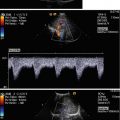
Spectral Doppler recordings of the flow in the renal arteries show a monophasic flow curve with high diastolic amplitude due to low peripheral vascular resistance (Figs. 10.2d, e, 10.3f, g, h and 10.6). These flow profiles can be found in all renal arteries from the hilus to the periphery of the renal parenchyma. From the anterior approach, a negative flow curve can be found (Fig. 10.2d, e), whereas from the lateral or the posterior view, a positive flow curve is typical (Fig. 10.3f, g, h). The high diastolic flow is typical of the renal circulation. It is caused by the Windkessel function of the aorta and the low peripheral resistance of renal vascular bed.

Fig. 10.6
(a) Flow velocities in the renal arteries of a 6-year-old boy. The flow velocities in the main renal artery (1st curve), the segmental artery (2nd curve), the interlobar artery (3rd curve) and the interlobular artery (4th curve) are displayed. From the hilus to the periphery, the flow velocities decrease. (b) Flow velocities in the interlobar (1st curve), segmental (2nd curve) and renal (3rd curve) artery of a 10-year-old girl
Most pathophysiologic situations which the abnormal or pathologic renal circulation influence the diastolic forward flow. All situations which can be interpreted as a leakage of the aortic Windkessel (such as a persistent ductus arteriosus Botalli, etc.) will cause a decrease of the diastolic amplitude. All pathophysiologic situations with increased vascular resistance in the renal periphery (such as acute renal insufficiency) will lead to swelling of the kidney and cause a decrease of the diastolic amplitude too.
10.4 Doppler Sonographic Flow Measurements in Renal Arteries Normal Values
If Doppler sonographic flow measurements in renal arteries are performed, it should be done in the following way:
1.
Use 2D imaging of the kidney. Obtain a qualitatively good 2D picture. Seek the corresponding artery were flow measurements can be performed (Fig. 10.2a).
2.
3.
Locate the Doppler line through the axis of the vessel with a minimal angle of incidence and place the sample volume within the vessel. The size of the sample volume should be adapted to the vessel size.
4.
5.
Measure the desired Doppler parameters (flow velocities and indices).
6.
Document the measurements.
Documentation should include a good colour Doppler picture which displays the location of the sample volume in the vessel, an artefact-free Doppler curve over several cardiac cycles and the measurements.
In our opinion, peak systolic, end-diastolic and time average velocity as well as the resistance index should be measured. Additionally, the end-systolic velocity, time average maximal velocity and the pulsatility index can optionally be measured or calculated.
As mentioned earlier, the measurement of the flow velocities should be preferred to the calculation of the indices, as perfusion of the organ can better be estimated from flow velocities (especially the time average velocity) than from indices.
10.4.1 Dependency of the Arterial Flow Velocities on the Location of the Sample Volume
Flow velocities decrease from the renal hilus to the periphery of the organ (Deeg et al. 2003). Flow velocities in the main renal arteries are highest, whereas flow velocities in interlobular and arcuate arteries are lowest (Fig. 10.6). From the renal hilus to the periphery, the flow velocities decrease. The peak systolic flow velocities in the segmental arteries are approximately one third lower than in the main trunk of the renal artery (Deeg et al. 2003). The flow velocities in the interlobar arteries are approximately one third lower than in the segmental arteries (Fig. 10.6) (Deeg et al. 2003). If absolute flow velocities are measured, the exact location of the sample volume of the pulsed Doppler device (renal, segmental, interlobar artery) has to be mentioned in the documentation. In the case of a large angle of incidence, angle correction should be performed.
10.4.2 Dependency of the Arterial Flow Velocities on Age
Beside the location of the sample volume biometric data influence the flow velocities in the renal arterial branches.
Flow velocities in the renal arteries are dependent on the age and weight of the patient. They are lowest in preterm infants and highest during school age and adolescence (Deeg et al. 2003). The greatest increase can be found in the first years of life, whereas in later childhood flow velocities show only a slight increase from school age to adolescence. The age dependency of the flow velocities in different renal arteries is summarised in Tables 10.1, 10.2, 10.3 and 10.4 and in Graphics 10.1, 10.2, 10.3, 10.4, 10.5, 10.6, 10.7 and 10.8.


Table 10.1
Normal values of the flow velocities and resistance indices in the renal arteries of healthy infants
Renal artery (n = 26) | Segmental artery (n = 26) | Interlobar artery (n = 18) | |
|---|---|---|---|
Age (weeks) | 7,3 ± 10,9 | 7,3 ± 15,1 | 9,4 ± 16 |
RR systolic (mmHg) | 68 ± 10 | 68,5 ± 10 | 70 ± 10 |
RR diastolic (mmHg) | 45 ± 6,3 | 45 ± 6,5 | 46 ± 6 |
V s (cm/s) | 51,5 ± 13,4 | 33 ± 8,0 | 19,5 ± 5,0 |
V es (cm/s) | 18,7 ± 7,1 | 12,4 ± 5,0 | 8,8 ± 2,9 |
V ed (cm/s) | 8,7 ± 5,0 | 6,2 ± 4,0 | 5,4 ± 3,5 |
TAV (cm/s) | 12,2 ± 4,6 | 7,8 ± 3,5 | 4,7 ± 1,7 |
RI | 0.82 ± 0,11 | 0,81 ± 0,12 | 0,73 ± 0,17 |
Table 10.2
Normal values of the flow velocities and resistance indices in the renal arteries of toddlers (≥1 and <6 years)
Renal artery (n = 31) | Segmental artery (n = 27) | Interlobar artery (n = 21) | |
|---|---|---|---|
Age (years) | 4,4 ± 1,1 | 4,3 ± 1,3 | 4,3 ± 1,1 |
RR systolic (mmHg) | 97 ± 9,8 | 95 ± 9,3 | 95 ± 8,3 |
RR diastolic (mmHg) | 61 ± 8,8 | 61 ± 8,7 | 62 ± 9,5 |
V s (cm/s) | 71,3 ± 13,5 | 43,6 ± 8,5 | 28,3 ± 6,8 |
V es (cm/s) | 32,2 ± 6,6 | 23,3 ± 6,4 | 16,0 ± 4,9 |
V ed (cm/s) | 20,3 ± 6,0 | 14,5 ± 4,2 | 9,9 ± 3,0 |
TAV (cm/s) | 19,2 ± 5,4 | 12,8 ± 3,2 | 9,3 ± 3,2 |
RI | 0.71 ± 0,08 | 0,67 ± 0,07 | 0,65 ± 0,08 |
Table 10.3
Normal values of the flow velocities and resistance indices in the renal arteries of school-age children (≥6 and <12 years)
Renal artery (n = 37) | Segmental artery (n = 34) | Interlobar artery (n = 28) | |
|---|---|---|---|
Age (years) | 9,1 ± 1,4 | 9,2 ± 1,3 | 9,3 ± 1,3 |
RR systolic (mmHg) | 105 ± 12,3 | 107 ± 11,5 | 105 ± 12 |
RR diastolic (mmHg) | 66 ± 8,0 | 66 ± 8,4 | 66 ± 8,6 |
V s (cm/s) | 80,0 ± 18,0 | 45,5 ± 9,1 | 27,9 ± 5,3 |
V es (cm/s) | 34,2 ± 9,6 | 23,4 ± 6,0 | 15,7 ± 3,6 |
V ed (cm/s) | 23,0 ± 7,7 | 15,5 ± 4,5 | 11,3 ± 2,7 |
TAV (cm/s) | 19,7 ± 6,5 | 11,8 ± 3,1 | 8,3 ± 1,9 |
RI | 0.71 ± 0,09 | 0,66 ± 0,08 | 0,58 ± 0,10 |
Table 10.4
Normal values of the flow velocities and resistance indices in the renal arteries of school-age children (≥12 and <18 years)
Renal artery (n = 30) | Segmental artery (n = 29) | Interlobar artery (n = 28) | |
|---|---|---|---|
Age (years) | 15,0 ± 1,9 | 14,7 ± 1,8 | 14,6 ± 1,8 |
RR systolic (mmHg) | 108 ± 8,0 | 110 ± 13,5 | 109 ± 13,9 |
RR diastolic (mmHg) | 69 ± 12,2 | 70 ± 12,2 | 69 ± 13,0 |
V s (cm/s) | 80,7 ± 13,7 | 46,8 ± 11,8 | 28,0 ± 6,1 |
V es (cm/s) | 35,1 ± 7,8 | 24,6 ± 6,2 | 16,0 ± 3,6 |
V ed (cm/s) | 24,9 ± 6,2 | 16,9 ± 4,1 | 11,2 ± 3,7 |
TAV (cm/s) | 20,7 ± 5,7 | 12,3 ± 3,0 | 8,2 ± 2,5 |
RI | 0.69 ± 0,06 | 0,63 ± 0,07 | 0,60 ± 0,06 |
Graphic 10.1
Normal values of peak systolic flow velocity (Vs) in the renal artery in dependency of age. Significant increase of the flow velocities with age (p < 0,0001)
Graphic 10.2
Normal values of peak systolic flow velocity (V s) in the interlobar artery in dependency of age. Significant increase of the flow velocities with age (p < 0,0001)
Graphic 10.3
Normal values of end–systolic flow velocities (V es) in the renal artery in dependency of age. Significant increase of the flow velocities with age (p < 0,0001)
Graphic 10.4
Normal values of end–systolic flow velocities (V es) in the interlobar artery in dependency of age. Significant increase of the flow velocities with age (p < 0,0001)
Graphic 10.5
Normal values of end–diastolic flow velocities (V ed) in the renal artery in dependency of age. Significant increase of the flow velocities with age (p < 0,0001)
Graphic 10.6
Normal values of end–diastolic flow velocities (V ed) in the interlobar artery in dependency of age. Significant increase of the flow velocities with age (p < 0,0001)
Graphic 10.7
Normal values of time average flow velocities (TAV) in the renal artery in dependency of age. Significant increase of the flow velocities with age (p < 0,0001)
Graphic 10.8
Normal values of time average flow velocities (TAV) in the interlobar artery in dependency of age. Significant increase of the flow velocities with age (p < 0,0001)
10.4.3 Dependency of the Arterial Flow Velocities on Weight
As the weight increases simultaneously with the age, there is also a strong dependency of an increase of the flow velocities with the weight of the patients. The correlation with the age however is better than with the weight (Deeg et al. 2003).
10.4.4 Dependency of the Resistive Index on Age
In contrast to the flow velocities, the resistive indices decrease with the age, the weight and the location of the sample volume.
The highest resistive indices could be found in the renal arteries in infants, the lowest in the interlobar arteries in adolescents. From the hilus to the renal periphery, the resistive indices fall in infants from 0,82 ± 0,11 to 0,73 ± 0,17 (Table 10.1), in toddlers from 0,71 ± 0,08 to 0,65 ± 0,08 (Table 10.2), in school-age children from 0,71 ± 0,09 to 0,58 ± 0,10 (Table 10.3) and in adolescents from 0,69 ± 0,06 to 0,60 ± 0,06 (Table 10.4) (Graphics 10.9 and 10.10) (Deeg et al. 2003).


Graphic 10.9
Normal values of the resistive indices (RI) in the renal artery in dependency of age. Significant decrease of resistive indices (p < 0,001)
Graphic 10.10
Normal values of the resistive indices (RI) in the interlobar artery in dependency of age. Significant decrease of the resistive indices (p < 0,001)
10.5 Doppler Sonographic Flow Measurements in the Renal Veins Normal Values
Flow measurements in renal veins are not routinely performed. Veins accompany the arteries from the hilus to the periphery. The main renal vein divides in several segmental veins which each gives rise to two interlobar veins. From the interlobar veins, several interlobular veins originate which drain the renal parenchyma. Flow can be measured in the main vein of the kidney, in the segmental and interlobar veins. The main stem of the renal vein is displayed at the hilus outside the renal parenchyma (Fig. 10.3a, b). The segmental veins can be obtained between the renal hilus and the pyramids (Fig. 10.3c, d). The interlobar veins run together with the interlobar arteries lateral to the pyramids (Fig. 10.3c, d).
With the help of colour Doppler, the veins can clearly be displayed, and the sample volume of the Doppler device can be located within the corresponding vein (Deeg et al. 2003).
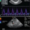
In healthy children, a continuous flow with a broad frequency spectrum can be shown in the renal veins. The flow profile is characterised by peaks and valleys which are caused by the cardiac cycle and by respiratory movements (Fig. 10.7). From the flow profile, the peak flow velocity (V max), the minimal flow velocity (V min) and the time average velocity (TAV) can be calculated (Figs. 10.7 and 10.8). Similar to the arterial resistive index, a venous resistive index can be calculated (V max − V min):TAV.


Fig. 10.7
(a) 2D image of the right renal vein from the anterior approach. The vein is compressed between the descending aorta (DAO) and the superior mesenteric artery (SMA). This leads to dilation of the left renal vein (LRV) called the nutcracker phenomenon. IVC inferior vena cava, VP portal vein. (b) Spectral Doppler of the flow measurement in the left renal vein from the anterior approach. Normal forward flow, with broad flow spectrum and slight alterations of the amplitude. (c) Colour Doppler imaging of the renal veins from the posterior approach. ILV interlobar vein, RV renal vein, SV segmental vein. (d–f) Flow measurements in the renal veins (posterior approach). The flow curves show a pulsatile venous flow which is influenced by atrial contractions and respiratory movements. From the periphery to the hilus, the flow velocities increase. (d) renal vein, (e) segmental vein, (f) interlobar vein
Fig. 10.8
(a) Doppler sonographic flow measurement in the left renal vein in an anterior approach. DAO descending aorta, PV portal vein, VCI inferior vena cava, VRli left renal vein. (b) Pulsed Doppler sonographic recording of the flow in the interlobar (1st curve), segmental (2nd curve) and renal (3rd curve) veins. The flow velocities increase from the periphery to the renal hilus
No normal values of the flow velocities and the resistive index within the renal veins have been published in the literature.
10.5.1 Dependency of the Venous Flow Velocities on the Location of the Sample Volume
In healthy infants, the flow velocities in the renal veins decrease from the renal hilus to the periphery. The highest flow velocities can be found in the renal veins, the lowest in the interlobar veins (Tables 10.5, 10.6, 10.7 and 10.8). Flow velocities decrease to one third from the renal vein to the segmental vein and to another third from the segmental vein to the interlobar vein.
Table 10.5
Normal values of the flow velocities in the renal veins of healthy infants
Renal vein (n = 20) | Segmental vein (n = 20) | Interlobar vein (n = 9) | |
|---|---|---|---|
Age (weeks) | 6,3 ± 7,8 | 5,2 ± 5,7 | 3,1 ± 15,3 |
RR systolic (mmHg) | 65,7 ± 9,5 | 68,4 ± 10,5 | 65 ± 11,8 |
RR diastolic (mmHg) | 45 ± 7,1 | 45,9 ± 6,8 | 45 ± 8 |
V max (cm/s) | 18 ± 6,7 | 12,7 ± 5,0 | 7,5 ± 2,2 |
V min (cm/s) | 11,7 ± 5,6 | 6,6 ± 4,4 | 4,8 ± 3,0 |
TAV (cm/s) | 6,8 ± 2,9 | 4,7 ± 1,9 | 3,5 ± 0,7 |
RI | 0,32 ± 0,29 | 0,45 ± 0,30 | 0,34 ± 0,40 |
Table 10.6
Normal values of the flow velocities in the renal veins of healthy toddlers (≥1 and <6 years)
Renal vein (n = 24) | Segmental vein (n = 15) | Interlobar vein (n = 11) | |
|---|---|---|---|
Age (years) | 4,45 ± 1,16 | 4,16 ± 1,0 | 4,4 ± 1,4 |
RR systolic (mmHg) | 96 ± 8,5 | 96 ± 9,1 | 99 ± 8,4 |
RR diastolic (mmHg) | 61 ± 8,3 | 60 ± 8,0 | 60 ± 9,2 |
V max (cm/s) | 23,4 ± 7,1 | 17,5 ± 3,5 | 10,5 ± 3,0 |
V min (cm/s) | 15,7 ± 5,6 | 10,3 ± 4,7 | 7,5 ± 2,2 |
TAV (cm/s) | 10,9 ± 3,2 | 7,4 ± 1,1 | 5,1 ± 1,0 |
RI | 0,32 ± 0,18 | 0,41 ± 0,20 | 0,26 ± 0,18 |
Table 10.7
Normal values of the flow velocities in the renal veins of healthy school-age children (>6 and <12 years)
Renal vein (n = 31) | Segmental vein (n = 26) | Interlobar vein (n = 19) | |
|---|---|---|---|
Age (years) | 9,3 ± 1,27 | 9,5 ± 1,2 | 9,6 ± 1,3 |
RR systolic (mmHg) | 105 ± 11,5 | 106 ± 10 | 109 ± 11 |
RR diastolic (mmHg) | 66 ± 8,3 | 65 ± 8,2 | 68 ± 7,8 |
V max (cm/s) | 24,8 ± 9,0 | 17,4 ± 4,0 | 12,3 ± 3,3 |
V min (cm/s) | 15,1 ± 6,7 | 11,5 ± 3,0 | 8,6 ± 2,3 |
TAV (cm/s) | 11 ± 3,9 | 8,0 ± 2,0 | 5,4 ± 1,3 |
RI | 0,37 ± 0,19 | 0,33 ± 0,18 | 0,27 ± 0,20 |
Table 10.8
Normal values of the flow velocities in the renal veins of healthy adolescents (>12 years)
Renal vein (n = 25) | Segmental vein (n = 26) | Interlobar vein (n = 16) | |
|---|---|---|---|
Age (years) | 15 ± 1,63 | 14,9 ± 1,8 | 14,5 ± 1,8 |
RR systolic (mmHg) | 109 ± 13 | 109 ± 13 | 111 ± 13 |
RR diastolic (mmHg) | 69 ± 11,9 | 70 ± 11,5 | 69 ± 11 |
V max (cm/s) | 26,6 ± 10,0 | 18,6 ± 4,7 | 12,8 ± 4,6 |
V min (cm/s) | 12 ± 5,3 | 12 ± 4,6 | 8,6 ± 2,8 |
TAV (cm/s) | 11,2 ± 4,4 | 7,8 ± 2,0 | 5,7 ± 1,7 |
RI | 0,53 ± 0,18 | 0,35 ± 0,20 | 0,30 ± 0,17 |
In infants, V max in the renal veins is 18 ± 6,7 cm/s, in the segmental veins 12,7 ± 5 cm/s and in the interlobar veins 7,5 ± 2,2 cm/s.
10.5.2 Dependency of the Venous Flow Velocities on the Age
From infancy to adolescence, a continuous increase of the flow velocities in the renal veins can be found (Tables 10.5, 10.6, 10.7 and 10.8). The lowest flow velocities can be found in infants, the highest in school age and adolescence. The fastest increase can be found in early childhood especially in toddlers.
Infants show a time average velocity of 6,8 cm/s, toddlers 10,9 ± 3,2 cm/s, school-age children 11 ± 3,9 and adolescents 11,2 ± 4,4 cm/s. In later childhood, no further increase could be found (Tables 10.5, 10.6, 10.7 and 10.8). In contrast to the flow velocities, the resistive index in the renal veins is relatively independent on age.
10.6 Pathologic Indications
The flow in the renal artery may be influenced by low volume state, cardiac insufficiency, shock and cardiovascular as well as by renal diseases.
10.6.1 Haemodynamic and Cardiovascular Diseases
10.6.1.1 Renal Perfusion in Low Volume State and Shock
Different haemodynamic alterations may influence blood flow in the renal arteries. In situations such as shock, the blood volume of the left ventricle and the contractility of the left ventricle are reduced. This causes low systolic flow and bad filling of the aortic Windkessel. Volume flow in the aorta is reduced which causes low volume flow in the abdominal arteries, especially the renal arteries. As the aortic Windkessel is not sufficiently filled in systole, diastolic flow is reduced. If renal swelling occurs, diastolic flow may be absent or even reverse too (Fig. 10.9).

Fig. 10.9
(a–c) Flow in the renal arteries of infants with low blood pressure and prerenal insufficiency after asphyxia. The image shows short systolic forward flow and missing diastolic flow (a) or diastolic backflow (b, c). The small systolic peak and the diastolic backflow are caused by bad contractility of the left ventricle caused by perinatal asphyxia. They cause low time average velocity and low volume flow responsible for oliguria or anuria
Low volume states also lead to missing or even retrograde diastolic flow (Fig. 10.10). Despite good contractility of the heart, the aortic Windkessel is filled insufficiently in systole which may cause diastolic backflow in the renal arteries due to early emptying (Fig. 10.10).

Fig. 10.10
(a, b) Doppler sonographic flow measurement in the renal artery of a patient with low intravascular volume: diastolic backflow caused by bad filling of the aortic ‘Windkessel’ in systole
10.6.1.2 Cardiac Malformations Which Influence Blood Flow in the Renal Arteries
Cardiovascular diseases which influence the flow in the renal arteries are obstructions of the left heart and malformations which cause a defect of the aortic Windkessel.
Cardiac malformations with a leakage of the aortic Windkessel are a great ductus arteriosus, a truncus arteriosus communis, an aorticopulmonary window, an aortic insufficiency and an aorticopulmonary shunt. These malformations may cause a significant decrease of the diastolic amplitude (Fig. 10.17). Large leakages of the aortic Windkessel may even cause diastolic backflow (Fig. 10.17b). The influence of these malformations on peripheral circulation is discussed in detail in the chapter on congenital heart disease.
Obstructions of the left heart are severe aortic stenosis, hypoplastic left heart syndrome, interruption of the aortic arch and coarctation of the aorta. These malformations cause a significant decrease of the systolic amplitude (Fig. 10.18). As pulsatility is reduced, the resistance index falls.
Renal and Urinary Tract Diseases Which Influence Blood Flow in the Renal Arteries
In this chapter, the uses of the various Doppler techniques for the diagnosis of renal vein thrombosis, renal arterial stenosis, infectious diseases of the kidney and urinary tract; in acute renal failure such as haemolytic-uraemic syndrome and acute rejection of a transplanted kidney; in obstructive and refluxive uropathy; in nephrolithiasis; and in renal and adrenal tumours are described (Deeg et al. 1990). The various indications are listed in Table 10.9.
Doppler sonography additionally can be used for the diagnosis of vascular diseases of the kidneys such as renal venous thrombosis and renal arterial stenosis.
10.6.1.3 Stenosis of the Renal Artery
Stenosis of the renal artery is a rare cause of arterial hypertension in infancy and childhood.
Stenosis or occlusion of the renal artery may cause renal ischemia and triggers the renin-angiotensin mechanism and causes hypertension. From a haemodynamic point of view, renal artery stenosis is considered significant if the diameter of the vessel is narrowed by 50–60 %.
Renal artery stenosis should be excluded in all children and adolescents with:
1.
Severe hypertension
2.
Rapidly accelerating hypertension
3.
Hypertension which is difficult to control despite suitable treatment
4.
Hypertension and deteriorating renal function
In all young patients with proven arterial hypertension, stenosis of the renal artery has to be excluded. The principal ultrasound criterion for renal artery stenosis is Doppler-detected elevation of flow velocities in the stenotic portion of the vessel. Flow velocities are increased in proportion to the severity of luminal narrowing. Doppler sonography therefore can be used to approximate the severity of the stenosis using the modified Bernoulli equation: Δp = 4 × v 2.
The investigation includes two-dimensional imaging, colour Doppler and pulsed and continuous wave Doppler of the flow velocities within the renal arteries.
2D Image
Direct visualisation of the stenosis usually is not possible as the demonstration of the complete course of the artery from the descending aorta to the renal hilus often is not possible due to overlying gas and the obesity of some patients.
Colour Doppler
Diagnosis can be made by the combined use of colour, PW and CW Doppler.
Low sensitivity (high Nyquist limit) of the colour Doppler device has to be used. The flow in the non-affected renal artery is displayed blue if an anterior approach is used (Fig. 10.2b, c). The affected stenotic artery shows a mosaic pattern in contrast to the healthy side (Fig. 10.11a). Narrowed areas detected with colour Doppler must be carefully surveyed with spectral or continuous wave Doppler to ensure that the maximal velocity is identified (Table 10.10).

Fig. 10.11
Renal arterial stenosis of the left renal artery in an 8-year-old boy with excessive arterial hypertension (Pictures (a–c) courtesy of E. Jung, Neunkirchen). (a) Colour Doppler of both renal arteries (transverse section through the upper abdomen). The normal flow in the non-stenotic right artery is displayed blue. AR re right renal artery. The flow in the stenotic left renal artery is displayed mosaic-like, indicating markedly increased flow. AR li left renal artery. (b) Doppler sonographic flow measurement in the normal right renal artery shows a normal flow profile and slightly elevated flow velocities (peak systolic flow velocity 1,55 m/s) caused by arterial hypertension. (c) Doppler sonographic flow measurement in the stenotic left renal artery shows pathologic turbulent flow (reversed flow displayed above the baseline) with an increase of the flow velocities up to 4,24 m/s corresponding to a gradient over the stenosis of 72 mmHg. (d) Damped flow curve in a distal localised segmental artery of a child with severe main stem stenosis. The flow curve shows very low flow velocities. The peak systolic flow velocity is 18 cm/s. The acceleration time is increased over 20 ms (Figure: Courtesy of J. Jüngert, Erlangen)
Table 10.9
Indications for Doppler sonography of the kidneys and urinary tract
Renal venous thrombosis |
Renal artery stenosis |
Infectious diseases of the kidney and urinary tract |
Glomerulonephritis |
Renal and adrenal tumours |
Cystic kidney disease |
Nephrolithiasis and nephrocalcinosis |
Obstructive and refluxive uropathy |
Ureteral jet |
Traumatic injury of the kidney |
Kidney transplantation |
Table 10.10
Doppler sonographic characteristics of renal arterial stenosis
Colour Doppler | Flow in ipsilateral artery mosaic-like |
Flow in contralateral artery normal (blue) | |
Prestenotic flow | Normal flow velocities |
Intrastenotic flow | Increase of flow velocities depending on severity of stenosis up to 300 % (>1,8 m/s) |
Quantification of the pressure gradient Δp = 4 × v 2 | |
Poststenotic flow | Broadening of frequency spectrum |
Backflow (mirror image) | |
Loss of spectral window due to turbulence | |
Dampening of flow curve | |
Jet phenomenon |
Pulsed Doppler
First of all, the flow in the non-affected artery should be measured (Fig. 10.11b). In the normal artery, normal flow profile and normal flow velocities can be measured (Fig. 10.11b). Only in severe hypertension the flow velocities in the normal artery are slightly elevated.
In the stenotic artery, flow before the stenosis has to be differentiated from flow within the stenosis and behind it.
Prestenotic Flow
Prestenotic normal flow velocities can be found. In comparison with the healthy side and with other abdominal arteries such as the celiac trunk, no significant difference exists. In cases of excessive hypertension, flow velocities may be increased similar as in other body arteries. Within the contralateral renal artery, normal flow profile and normal flow velocities can be shown (Fig. 10.11b). Only in cases of excessively elevated blood pressure flow velocities may be increased.
Intrastenotic Flow
Within the stenosis, a significant increase of the flow velocities can be found. The increase is dependent on the grade of the stenosis. According to the continuity equation of Bernoulli, the flow velocities increase if the cross-sectional area decreases.

A is the cross-sectional area; V is the flow velocity.
In significant obstructions, the peak systolic flow velocities increase over more than 1,8 m/s up to 300 % of the normal values. In severe stenoses, the intrastenotic flow velocities are sometimes so high that they cannot be measured with spectral Doppler. In these cases, continuous wave Doppler, which is not limited by high flow velocities, should be used (Fig. 10.11c). Usually abdominal ultrasound programmes are only equipped with spectral Doppler. If cardiologic software is used, even very high peak systolic flow velocities, such as in severe stenoses, can be measured and quantified (Fig. 10.11c).
For the exact quantification of the peak systolic flow velocity, accurate assignment of the angle of incidence is essential. As mentioned earlier, the Doppler-to-vessel angle should not exceed 45° to ensure that the velocity information is accurate.
The Bernoulli equation Δp = 4 × V 2 allows quantification of the pressure gradient along the stenosis (Table 10.11).
Table 10.11
Flow characteristics of stenosis of the renal artery far behind the stenosis
Flow velocities ↓ |
Acceleration slope ↓ |
Acceleration time ↑ |
Deceleration slope ↓ |
Deceleration time ↑ |
PI and RI ↓ |
Poststenotic Flow
Immediately behind the stenosis typically a jet phenomenon can be found. Additionally, mirror image of the flow and spectral broadening characteristic of turbulent flow can be shown. A spectral window typical of laminar flow cannot be seen.
Far behind the stenosis, a dampened flow curve with low flow velocities can be found within the interlobar and interlobular arteries in comparison to the non-affected side (Fig. 10.11d). The most important downstream manifestations of renal artery stenosis are the absence of an early systolic peak, a prolonged acceleration time and a reduced acceleration index (Fig. 10.11d).
Stenosis can occur not only in the main stem of the renal artery but also in the peripheral branches. These stenoses can be detected, if the sensitivity of the colour Doppler device is decreased (high PRF or Nyquist limit). Only arteries with a very high flow are displayed, whereas all arteries with normal low flow velocities are depressed (Fig. 10.12a). In a second step, the sample volume of the Doppler device is placed in the artery which is displayed with colour Doppler (Fig. 10.12b). In patients with tuberous sclerosis, peripheral interlobar arteries may be compressed by angiomyolipomas and cause hypertension (Fig. 10.12). Low sensitivity may show the narrowed artery (Fig. 10.12a), whereas pulsed Doppler shows the increased flow velocities (Fig. 10.12b).

Fig. 10.12
Stenosis of an interlobar artery in a patient with tuberous sclerosis and angiomyolipomas of the kidney. (a) Colour Doppler displays only the stenotic interlobar artery. Due to chosen high pulse repetition frequency of 69 m/s and low sensitivity of the colour Doppler device, no other artery beside the stenotic one is displayed. (b) Doppler sonographic flow measurement within the stenotic interlobar artery shows an increased flow with a peak systolic flow velocity of 1,51 m/s
Different parameters have been used for the diagnosis of renal artery stenosis: the difference between the resistive index of both renal arteries (Riehl et al. 1997; Schwerk et al. 1994), the estimation of the acceleration time and the acceleration (Ripolles et al. 2001) and the estimation of the peak systolic flow velocities in renal and interlobar arteries (Brun et al. 1997; Li et al. 2006).
Schwerk et al. (1994) and Riehl et al. (1997) compared the resistance index in kidneys with renal artery stenosis with the contralateral non-affected kidney: The RI in kidneys with renal artery stenosis was significantly reduced. A ∆ RI of 8 % between both kidneys yields a sensitivity of 92,5 % and a specificity of 95,7 % (Riehl et al. 1997). Ripolles et al. (2001) found an increased acceleration time (time till peak systolic flow velocity is reached) of >80 ms and a decreased acceleration ≤1 m/s2 adults.
Due to the low frequency of renal artery stenosis in infancy and childhood, only few reports of the use of renal Doppler sonography for the diagnosis of renal artery stenosis in infancy and childhood in literature exist. Brun et al. (1997) investigated 22 hypertensive children. He suggests that renal arterial stenosis should be suspected if the peak systolic flow velocity in the renal artery exceeds 1,8–2 m/s (Brun et al. 1997).
Beside the peak systolic flow velocity, a renal/aortic ratio exceeding 3,3–3,5 is the most universally accepted Doppler criterion for the diagnosis of renal artery stenosis. The latter is the ratio of peak systolic flow velocity in the stenotic portion of the renal artery divided by the peak systolic flow velocity in the aorta at the renal level. Pellerito and Zwiebel (2005) uses the renal/aortic ratio as the primary criterion for diagnosis of renal arterial stenosis. The renal/aortic ratio compensates for haemodynamic variability between patients.
An easy method with great sensitivity is the estimation of the ratio between the peak systolic flow velocity in the renal artery and the interlobar artery. In significant renal arterial stenosis of 50 % and more, the ratio exceeds five (Li et al. 2006). The combination with a peak systolic flow velocity less than 15 cm in the interlobar arteries provides the best diagnostic efficiency (Li et al. 2006). The investigations of Li were performed in adults. As the flow velocities in school age and adolescence do not differ significantly from adulthood these values can be used in paediatric patients over the age of 6 years.
Doppler sonographic estimation of renal artery stenosis in children depends on the skill of the operator and is dependent on experience. In obese children and due to overlying gas, the renal arteries cannot be displayed in all patients. In these patients, intrarenal Doppler waveforms should be measured from the dorsal or dorsolateral approach in segmental or interlobar arteries. Renal artery stenosis can cause pulsus tardus and parvus in intrarenal arteries (Handa et al. 1988; Nichols et al. 1984; Patriquin et al. 1992; Stavros et al. 1992). According to Stavros, pulsus tardus and parvus in segmental arteries is an excellent indirect method for diagnosis of renal arterial stenosis. This technique however is not able to differentiate severe stenosis from occlusion with collateral arteries (Stavros et al. 1992). Intrarenal Doppler alterations can only be found in severe stenosis exceeding more than 70 % of vessel diameter (Pellerito and Zwiebel 2005). The detection of abnormal waveforms confirms the haemodynamic significance of main stem renal artery stenosis. Damped intrarenal waveforms may indicate occult stenosis in the main renal artery or in a segmental artery (Fig. 10.11d). This is particularly important when direct visualisation of the artery is technically limited.
Other problems are abnormal and accessory renal arteries and distal lesions that may be missed (Brun et al. 1997).
10.6.2 Renal Venous Thrombosis
Although renal vein thrombosis (RVT) can occur at any age, it is more frequent in neonatology. 80 % of all RVT occur in neonatology (Andrew and Brooker 1996). Risk factors for RVT are asphyxia, shock, congenital heart disease, dehydration, polycythaemia, sepsis, diabetes of the mother and difficult delivery of a large infant. Other risk factors are umbilical artery catheterisation, surgery and trauma. Genetic factors, such as inherited prothrombotic states, may play an important role in the development of RVT.
10 % of RVT are associated with adrenal haemorrhage. RVT more often affects the right kidney, as the right side lacks venous collaterals. The incidence of RVT is 2,2 cases per 100,000 live births, with a sixfold higher rate in preterm neonates (Böbenkamp et al. 2000).
Renal venous thrombosis (RVT) can be divided into adult and infantile forms. Adult RVT is characterised by a thrombus in the renal vein, whereas in infantile RVT thrombosis of the small veins of the kidney can be found. Clotting starts in the small intrarenal veins during venous stasis. Microthrombi spread distally and involve the renal cortex and medulla extending into larger veins.
RVT can occur unilaterally and bilaterally. Bilateral disease is found in up to 20 % (Böbenkamp et al. 2000). In 30 % RVT may extend from the renal periphery into the inferior vena cava.
Typically, RVT manifests with haematuria, flank mass, thrombocytopenia and alterations of blood pressure. Other clinical and laboratory signs are oliguria, haemolytic anaemia, metabolic acidosis and azotaemia.
Diagnosis
The imaging modality of choice is the combination of 2D ultrasound and Doppler sonography (duplex sonography). 2D images display the alterations of renal anatomy, Doppler sonography the changes of renal perfusion. Flow changes have to be differentiated in arterial and venous alterations. Sonography confirms the diagnosis with an accuracy of 92 % percent (Ricci and Lloyd 1990).
2D Image
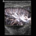
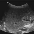
In a newborn with gross haematuria, always renal venous thrombosis has to be excluded. The morphologic alterations depend on the stage in which the investigation is performed. Greyscale images show an increased kidney size in comparison to healthy infants and to the non-affected kidney in unilateral disease (Fig. 10.13). To evaluate the size of the kidney, the volume of the organ should be measured using the modified ellipsoid formula (length × depth × width/2). In unilateral disease, the affected kidney is significantly larger in comparison with the healthy organ. In the acute phase of the disease, the renal medulla is swollen and appears echo poor (Hibbert et al. 1997). Initial diagnostic features include renal enlargement, echo poor medullary pyramids, subsequently loss of corticomedullary differentiation, reduced echogenicity around the affected pyramids and echogenic bands at the extreme apex of the pyramid (Fig. 10.13a, b) (Elsaify 2009). Lateral to the pyramids echogenic streaks corresponding to the thrombus formation in the interlobar veins can be found in the acute phase of the disease (Elsaify 2009; Hibbert et al. 1997). The echogenic streaks persist only for a few days before they disappear (Hibbert et al. 1997). In the later stage of the disease, the echogenicity of the enlarged kidney is increased, and the corticomedullary differentiation is lost (Fig. 10.13). The sonographic features vary according to the severity, the extent of the thrombosis, the development of collateral circulation and the stage of renal vein thrombosis (Elsaify 2009). The changes of the 2D image however are nonspecific and can be found in other renal diseases of the newborn too. Therefore, additionally Doppler sonographic flow measurements in the renal vessels should be performed.

Fig. 10.13
(a, b) Renal venous thrombosis in a neonate with macrosomia after traumatic delivery. The size of the kidney is markedly increased with a length of 6,8 cm and a depth of 3,2 cm (markers). The echogenicity is focally increased with bad corticomedullary differentiation and inhomogeneous echogenic stripes laterally to the renal pyramids (representing thrombosed interlobar arteries). (a) longitudinal section, (b) transverse section. (c) Colour Doppler of the flow in the kidney. Although sensitive settings of the colour Doppler device are chosen, only minimal flow can be shown at the renal hilus
Doppler Sonography
Doppler sonographic changes in RVT are more specific and typical of RVT. In unilateral cases, comparison of the flow in both organs should be used.
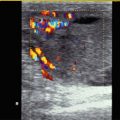
Colour Doppler shows diminished or even absent flow, although low flow settings (low PRF, low wall filter, high gain) are used (Figs. 10.13c and 10.14). In unilateral disease, flow in the healthy kidney can be used for comparison (Fig. 10.14). In severe cases, no flow can be demonstrated although appropriate sensitive flow settings of the Doppler device have been used (Fig. 10.14a–c).

Fig. 10.14
(a) Colour Doppler of the vascularisation in renal venous thrombosis. Although sensitive flow settings have been chosen, only few intrarenal vessels can be shown. (b, c) Power Doppler shows nearly no intrarenal vascularisation in an infant with unilateral renal venous thrombosis
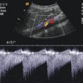
Pulsed Doppler recordings of the flow in the renal vessels have to be differentiated in arteries and veins. As mentioned earlier, the disease typically starts in the small intrarenal veins when venous stasis occurs. Higher resistance indices in renal arteries and absent, steady or less pulsatile venous flow on the affected side compared with flow in the contralateral kidney are helpful Doppler signs (Fig. 10.15) (Elsaify 2009).

Fig. 10.15
(a–d) Pulsed Doppler sonographic flow measurements in the renal artery in the non-affected kidney (a) and in two neonates with renal venous thrombosis (b–d). (a) Normal vascularisation by power Doppler and normal flow profile and flow velocities in the non-affected kidney (high diastolic amplitude). (b) Pathologic flow profile with systolic forward flow and holo-diastolic backflow due to almost complete obstruction of the peripheral circulation. (c, d) Pathologic flow in an intrarenal artery of an other patient with RVT. Colour Doppler reveals only few intrarenal vessels. Pulsed Doppler shows pathologic biphasic flow with very low flow velocities. Time average flow velocity and perfusion approximates zero. (e) Normal flow profile and normal flow velocities in an extrarenal artery, the celiac trunk of an infant with renal venous thrombosis
Veins: If large parts of the renal periphery are occluded, no flow can be shown by colour Doppler (Fig. 10.13c). In the larger renal veins at the renal hilus, pulsed Doppler recordings show minimal venous flow or no flow signals (Fig. 10.14a).
Arteries: Flow in the renal artery is reduced. In severe RVT, systolic forward flow and diastolic backflow can be found (Fig. 10.15b–d) (Deeg et al. 1985). Due to total or subtotal obstruction of the renal periphery, the peripheral resistance is markedly increased. This causes a venous outlet obstruction and a retrograde diastolic flow in the renal arteries (Fig. 10.15b). In severe cases, no other artery beside the main stem of the renal artery can be demonstrated by Doppler sonography. In partial thrombosis, focal perfusion may be shown by colour Doppler. In these cases, pulsed Doppler reveals a decreased diastolic forward flow with an increase of the resistance index (Cai et al. 2007). Cai investigated ten infants with RVT: He found a negative diastolic flow only in 4 of 11 affected kidneys (36 %). The other kidneys were partially affected and showed an increased resistance index (mean 0,85) (Cai et al. 2007).
Doppler sonographic flow measurements are very helpful for further controls. Under treatment with heparin or thrombolytic therapy with r-TPA or urokinase flow may be re-established. Colour and pulsed Doppler show reappearing vessels and flow (Fig. 10.16a). Depending on the severity of the disease, the kidney shrinks and gets more and more atrophic (Fig. 10.16b). Kidney atrophy is already present at 1 year of age in two thirds of all patients with sonographic diagnosis of RVT (Böbenkamp et al. 2000). Persistent renal imaging abnormalities were present in more than 80 % of all affected infants (Mocan et al. 1991).

Fig. 10.16
 Transcranial Colour Doppler Sonography (TCDI)
 Physical and Technical Principles of Doppler Sonography
 Doppler Sonography of the Abdominal Vessels
 Doppler Sonography of the Scrotum
 Cardiovascular Diseases Which Influence the Flow in the Extracardial Arteries
 Doppler Sonography of the Liver in Infants and Children


(a) Reopening of the peripheral circulation 1 week after conservative treatment with heparin. Colour Doppler shows multiple intrarenal vessels. (b) Although reopening of peripheral circulation occurred large parts of the affected kidney showed cystic transformation and degeneration. As the child developed gross haematuria, the kidney had to be removed. (c) Anatomic specimen of the kidney. Approximately 2/3 of the kidney are necrotic
Related posts:
Transcranial Colour Doppler Sonography (TCDI)
Physical and Technical Principles of Doppler Sonography
Doppler Sonography of the Abdominal Vessels
Doppler Sonography of the Scrotum
Cardiovascular Diseases Which Influence the Flow in the Extracardial Arteries
Doppler Sonography of the Liver in Infants and Children
Stay updated, free articles. Join our Telegram channel
Full access? Get Clinical Tree
