Fig. 3.1
The arterial circle of Willis and the vertebrobasilar arterial system. The ophthalmic artery (OA) originates from the internal carotid artery in the cerebral segment. The internal carotid artery bifurcates into the anterior cerebral artery and the middle cerebral artery, which normally is the larger branch. This segment of the ICA is the origin of the ophthalmic artery, the posterior communicating artery and the anterior choroidal artery. The posterior communicating artery (PCoA) courses posteriorly and medially from the internal carotid artery to join the posterior cerebral artery (PCA). The middle cerebral artery (MCA) is the blood supply to most of the lateral surface of the cerebral hemisphere (see Fig. 3.2). From its origin, the MCA extends laterally and horizontally in the lateral cerebral fissure (see Fig. 3.2). The MCA either bifurcates or trifurcates, and the terminal branches of the MCA anastomose with terminal branches of the anterior cerebral and the posterior cerebral arteries building ‘watersheds’ of the cerebral perfusion (see Fig. 3.2). The two anterior cerebral arteries (ACA) course antero-medially to the interhemispheric fissure. The proximal, horizontal segment of the anterior cerebral artery is termed the A1 segment and is connected to the contralateral A1 segment by the anterior communicating artery. The anterior cerebral arteries turn upwards in the interhemispheric fissure. The segment of the ACA from the anterior communicating artery to the distal anterior cerebral artery bifurcation is termed the A2 segment. The basilar artery (BA) is formed by the two vertebral arteries and is variable in its course, size and length. The posterior cerebral artery (PCA) courses anteriorly and laterally. The segment of PCA from its origin to its junction with the posterior communicating artery is named P1, and the portion of the vessel extending posteriorly to the midbrain is called the P2 segment. (Drawing by Blankvisual, Thun, Switzerland)

Fig. 3.2
Perfusion areas of the great intracranial arteries and resulting watersheds of arterial supply (enclosed by dashed lines). 1 basilar artery, 2 vertebral artery, 3 branches of the posterior cerebral artery, 4 terminal branches of the middle cerebral artery and 5 terminal branches of the anterior cerebral artery. (Drawing by Blankvisual, Thun, Switzerland)
The circulus arteriosus Willisii works as an anastomotic ring permitting (in most patients) shunting of blood between the cerebral hemispheres (by the ACoA) and between the anterior and posterior systems (by the PCoAs). Variations of the circle of Willis are quite common. A classic completely ‘normal’ circle of Willis is found in only approximately 20–40 % of paediatric patients (Ardakani et al. 2008; Krishnaswamy et al. 2010).
The Doppler evaluation of the intracranial arteries is performed with a low-frequency (2–3 MHz) sector imaging transducer.
The measured flow velocities are only correct if there is a zero degree angle between the vessel and the Doppler beam. In vessel segments where this cannot be achieved, angle correction of the flow velocities should be done, knowing the principle error sources of this method.
Many investigators are, as us, reporting results using peak systolic and end diastolic velocities instead of the traditionally accepted mean velocities (TAV = time average velocity and TAMX = time average peak velocity).
Each institution will have to decide which velocity values have to be documented and set the diagnostic criteria accordingly for the different clinical situations.
3.1.2 Investigation Technique and Normal Findings
3.1.2.1 Patient Positioning
TCDI examinations are regularly performed with the patient in the supine position. The supine position allows access to the transtemporal, transorbital and submandibular windows. The suboccipital examination can be performed with the patient lying supine and the head turned to one side.
3.1.2.2 TCDI Examination Windows
A TCDI examination can be done through the following four sound windows (Figs. 3.3 and 3.4):


Fig. 3.4
A schematic of the circle of Willis visualised from the transtemporal axial approach. Middle cerebral artery (M1 and M2), anterior cerebral artery (A1 and A2) and posterior cerebral artery (P1 and P2); the mesencephalon forms a ‘butterfly’ structure in the centre of the image (arrow) representing an important anatomic landmark for the investigation. (Drawing by Blankvisual, Thun, Switzerland)
Transtemporal
Transorbital
Suboccipital
Submandibular
In most cases, investigations are performed using the transtemporal window (Coley 2012).
In younger children, in addition, an approach through the closed great fontanelle is often possible especially for the investigation of the anterior cerebral arteries. This approach is identical to the transfontanellar windows and has been discussed there.
The depth ranges (mm) and the age-related normal mean peak velocities (TAMX cm/s) of the intracranial arteries evaluated by each approach are given in Table 3.1. Table 3.2 shows the age-dependant normal values of the other flow velocities in children and adult patients. The depth ranges are useful for a preset of the transducer in non-cooperative patients leading to a faster investigation. In general, anatomic landmarks (see Fig. 3.1) should be used to identify the target vessels.
Table 3.1
Acoustic windows, targeting depth for the different vessels and normal peak mean (TAMX) flow velocities ± standard deviation
Window | Artery | Depth (mm) | Age 1–2.9 years TAMX | Age 3–5.9 years TAMX | Age 6–9.9 years TAMX | Age 10–16.9 years TAMX | Adults TAMX (cm/s) |
|---|---|---|---|---|---|---|---|
Transtemporal | Middle cerebral | 20–67 | 85 ± 10 | 94 ± 10 | 97 ± 9 | 81 ± 11 | 62 ± 12 |
(or transfontanellar) | Anterior cerebral | 40–80 | 55 ± 13 | 71 ± 15 | 65 ± 13 | 56 ± 14 | 50 ± 11 |
Terminal internal | 40–67 | 81 ± 8 | 93 ± 9 | 93 ± 9 | 79 ± 12 | 39 ± 9 | |
Carotid | |||||||
Posterior cerebral (PCA1) | 35–80 | 50 ± 17 | 56 ± 13 | 57 ± 9 | 50 ± 10 | 39 ± 10 | |
Posterior communicating | 45–85 | ||||||
Anterior communicating | 45–72 | ||||||
Transorbital | Ophthalmic | 20–60 | 21 ± 5 | ||||
Internal carotid (siphon) | 20–80 | 75 ± 10 | 91 ± 11 | 89 ± 11 | 77 ± 14 | 47 ± 10 | |
Suboccipital | Vertebral | 20–85 | 38 ± 10 | ||||
Basilar | >60 | 51 ± 6 | 58 ± 6 | 58 ± 9 | 46 ± 8 | 41 ± 10 | |
Submandibular | Distal internal | 15–70 | 81 ± 8 | 93 ± 9 | 93 ± 9 | 79 ± 12 | 37 ± 9 |
Carotid |
Table 3.2
Resistance index (RI) and normal flow velocities ± standard deviation
Velocity (cm/s) ± standard deviation | Artery | Age 1–2.9 years | Age 3–5.9 years | Age 6–9.9 years | Age 10–17.9 years | Adults |
|---|---|---|---|---|---|---|
Vs | Middle cerebral (MCA1) | 124 ± 10 | 147 ± 17 | 143 ± 13 | 129 ± 17 | 110 ± 28 |
Anterior cerebral | 81 ± 19 | 104 ± 22 | 100 ± 20 | 92 ± 19 | 79 ± 21 | |
Internal carotid | 118 ± 24 | 144 ± 19 | 140 ± 14 | 125 ± 18 | ||
Posterior cerebral (PCA1) | 67 ± 18 | 84 ± 20 | 82 ± 11 | 75 ± 16 | 71 ± 16 | |
Internal carotid (siphon) | 114 ± 21 | 138 ± 14 | 132 ± 17 | 120 ± 21 | ||
Basilar | 71 ± 6 | 88 ± 9 | 85 ± 17 | 68 ± 11 | ||
Ved | Middle cerebral | 65 ± 11 | 65 ± 9 | 72 ± 9 | 60 ± 8 | 49 ± 14 |
Anterior cerebral | 40 ± 11 | 48 ± 9 | 51 ± 10 | 46 ± 11 | 35 ± 11 | |
Internal carotid | 58 ± 5 | 66 ± 8 | 68 ± 10 | 59 ± 9 | ||
Posterior cerebral (PCA1) | 36 ± 13 | 40 ± 12 | 42 ± 7 | 39 ± 8 | 33 ± 14 | |
Internal carotid (siphon) | 55 ± 12 | 62 ± 8 | 67 ± 11 | 58 ± 12 | ||
Basilar | 35 ± 6 | 41 ± 5 | 44 ± 8 | 36 ± 7 | ||
RI | Middle cerebral | 0.47 ± 0.05 | 0.55 ± 0.05 | 0.50 ± 0.05 | 0.53 ± 0.05 | 0.56 ± 0.06 |
Anterior cerebral | 0.55 ± 0.05 | 0.57 ± 0.05 | 0.57 ± 0.05 | 0.58 ± 0.05 | 0.56 ± 0.07 | |
Internal carotid | 0.52 ± 0.05 | 0.60 ± 0.05 | 0.55 ± 0.05 | 0.58 ± 0.05 | ||
Posterior cerebral (PCA1) | 0.55 ± 0.05 | 0.58 ± 0.05 | 0.55 ± 0.05 | 0.55 ± 0.05 | 0.54 ± 0.06 | |
Internal carotid (siphon) | 0.57 ± 0.05 | 0.63 ± 0.05 | 0.55 ± 0.05 | 0.58 ± 0.05 | ||
Basilar | 0.55 ± 0.05 | 0.60 ± 0.05 | 0.55 ± 0.05 | 0.57 ± 0.05 |
3.1.2.3 Transtemporal Window
The transtemporal investigation is performed with the patient in the supine position and the head straight to avoid obstruction of the venous return. The transducer is placed anterior to the ear on the temporal bone cephalad to the zygomatic arch. The transtemporal examination window varies in size and location with each patient and may vary in an individual from one side to the other (Coley 2012). The transtemporal investigation is not possible in up to 10 % of the paediatric population when performing a TCDI examination and is more difficult to find in young adults, in Africans and in children after implantation of cerebrospinal shunt systems. In these patients, the other acoustic windows (suboccipital, orbital) may be used.
The transducer should be angled slightly superior in an axial imaging plain. This orientation of the transducer produces an image that is a transverse oblique view of the anterior and posterior intracranial circulation.
Additionally, the transducer can be rotated by 90° to obtain a transverse coronal image. This to our experience can in many cases produce a much better visualisation of the internal carotid arteries and the distal segments of the MCA (see Fig. 3.5).

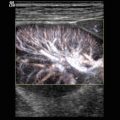
Fig. 3.5
Pulsed Doppler spectral signal from the middle cerebral artery (MCA) in a 17-year-old boy. The sample volume is placed in the right MCA (coded red)
The ipsilateral hemisphere is at the top and the contralateral hemisphere at the bottom of the image, with anterior being to the left and posterior to the right side, similar to the images of computed tomography and axial MRI.
The contralateral skull produces echoes near the bottom of the image. The bitemporal diameter of the skull varies with age from about 7–9 cm in neonates to about 11–13 cm in young adults (Bode 1988).
Visualisation of the contralateral arterial system is possible in many paediatric patients, but each brain hemisphere should be separately studied through an ipsilateral window to obtain the best (near-zero) vessel-to-transducer angle.
Afterwards the transducer is angled slightly inferior to identify the anatomic landmarks. The strongest echo extending anteriorly is the lesser wing of the sphenoid bone, and the petrous ridge of the temporal bone extends posteriorly, If the transducer is rotated by 90° at the transtemporal window, a coronal image is generated (see Figs. 3.6 and 3.7).


Fig. 3.6
The circle of Willis investigated from a transtemporal approach. Middle cerebral artery (MCA), anterior cerebral artery (ACA) and posterior cerebral artery (PCA) are shown in the axial plane (a) (Image courtesy Prof. K.H. Deeg); (b) in teenagers and adults, a complete investigation of the circulus is seldom possible due to the much more torcular course of the arteries; in these patients, the arteries have to be documented in different planes. In a standard documentation, the left side of the image shows the front of the patient’s head and the right side the back of the patient’s brain (using the axial plane). The upper image side represents the nearer cerebral hemisphere in both planes. ME mesencephalon
Fig. 3.7
Circle of Willis from the transtemporal window colour Doppler energy (CDE) mode. If the transducer is rotated by 90° at the transtemporal window, a coronal image is generated. In this transtemporal coronal view, the internal carotid artery and the distal parts of the MCA are shown
It is important to remember that the transcranial colour Doppler images are only maps in two dimensions. Tortuous intracranial arteries cannot be displayed along their whole length as a continuous colour pathway, and repeatedly crossing the image plane even may suggest artificial stenosis (see Sect. 3.1.4.1).
3.1.2.4 Suboccipital Window
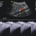
When investigating the vertebrobasilar system using the suboccipital window, the patient should be laying the head bowed sligthly towards the chest because this position increases the acoustic window between the skull and the atlas. The transducer is placed on the neck inferiorly to the nuchal crest, with the ultrasound beam directed towards the bridge of the patient’s nose (see Fig. 3.8).

Fig. 3.8
(a, b) Transducer position using the suboccipital window. The arterial flow is away from the transducer. The colour map is used to position the Doppler sample volume in the vertebral artery (a left image) or in the basilar artery (b right image). In a standard documentation scheme, the left image side shows the left side of the patient’s brain. (Drawing by Blankvisual, Thun, Switzerland). (c) TCDI using the suboccipital windows. Both vertebral arteries and the basilar artery are forming characteristic y-sign. Arterial flow is away from the transducer and therefore coded in blue
The depth range of the image should be set for 10–12 cm. The basilar artery is often tortuous so that calliper variations in the colour map should only with caution be interpreted as stenosis.
3.1.2.5 Transorbital Window
The transorbital investigation shows the ophthalmic artery and the carotid siphon. In practice in the paediatric age group, this window is more often used to investigate the ophthalmic artery, e.g. as reference vessel. The current FDA maximum acoustic output allowable levels (derated) for ophthalmic imaging are a spatial peak temporal average (SPTA) intensity of 17 mW/cm2 and reduced power settings with a mechanical index not to exceed 0.23 to prevent ocular injury (Coley 2012). The examination is done with the patient in the supine position, and the transducer placed on the closed eyelid.
A better image of the anatomic structures and the ophthalmic artery may be obtained using a higher-frequency (7.5–10 MHz) linear array transducer.
The imaging plane should be directed medially, towards the nose. Examination of either eye should generate an image with medial (nasal) on the left side and temporal on the right side of the image. The carotid siphon is located at a depth of 40–80 mm (see Table 3.1). To evaluate the ophthalmic artery (OA), the depth setting of the Doppler sample volume should be in the range of 20–60 mm (see Table 3.1). The OA is generally identified adjacent to the optic nerve, showing a high pulsatility and a dicrotic flow profile.
3.1.2.6 Submandibular Window
The submandibular window is a continuation of the duplex imaging evaluation of the extracranial distal internal carotid artery. The transducer is placed at the angle of the mandible and adjusted medially and cranially towards the carotid canal. The transducer’s imaging plane is adjusted in a sagittal direction. The submandibular window is rarely used in paediatric patients.
3.1.3 Intracranial Venous Anatomy
The intracranial veins are mostly examined in the supine position using the transtemporal window. Intracranial veins and sinuses show a low pulsatile flow with a maximal systolic blood flow velocity of around 10 cm/s in younger children and around 20 cm/s in children older than 2 years (see Table 3.3). The flow velocities show a respiratory modulation in the great sinus, whereas the flow in the small veins, in the vein of Galen and in the straight sinus is nearly continuously.
Table 3.3
Normal values for the flow velocities in the great intracranial veins and sinus
Vein | Time average peak flow velocity (cm/s) | |
|---|---|---|
Children | Adults | |
Right internal cerebral vein | 3.4 ± 0.2 | 14 ± 3 |
Left internal cerebral vein | 3.2 ± 0.3 | 14 ± 3 |
Transverse sinus | 24 ± 6 | |
Great vein of Galen | 4.3 ± 0.7 | |
Straight sinus | 5.9 ± 1.0 | 26 ±6 |
Superior sagittal sinus | 9.2 ± 1.1 | |
In the axial plane (see Figs. 3.9, 3.10 and 3.11), the basal veins follow the course of the PCA and are visualised adjacent and superior to the P2 segment. The detection rate of the intracranial veins by TCDI is known to be about 70–80 %. Directing of the transducer to the level of the third ventricle visualises the vein of Galen in the midline. If the transducer is rotated upwards, the straight sinus can be seen. The detection rate of the intracranial veins by TCDI is known to be about 70–80 %.


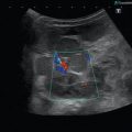
Fig. 3.9
Schematic of the transorbital investigation window (a) (Drawing by Blankvisual, Thun, Switzerland) and (b) colour map of the transorbital investigation; the Doppler sample volume is placed in the orbital artery (OA)
Fig. 3.10
Schematic drawing of venous anatomy of the basal cerebral veins, great vein of Galen and transverse, superior sagittal and straight sinus. (Drawing by Blankvisual, Thun, Switzerland)
Fig. 3.11
TCDI examination of the venous system (right internal cerebral vein) using a transtemporal window. ME mesencephalon
In the rare published studies about the flow velocities in the intracranial veins, these flow velocities show a similar age dependency as the arterial flow velocities.
At the moment, not enough data is present concerning normal values of the flow velocities in the intracerebral veins in children.
The sparse known values are summarised in Table 3.3.
In cases of known intracranial anomalies like the vein of Galen AVM, the absolute flow velocities in the draining venous system are clearly increased and can be used to monitor therapy. In many other cases of venous disease, the normal values are less reliable; this is in part due to the insonation angle and the errors due to the necessary angle correction using the transtemporal window.
Therefore, the most useful TCDI results regarding the intracranial venous system are from investigating the presence and direction of flow in an intracranial vein, comparing velocities from different sample volume depths from the same vein or sinus and comparing the velocities from the different veins (sides) within a patient. Bilateral symmetric disease is difficult to diagnose by venous TCDI.
Using the transfontanellar approach, the intracranial venous system can be imaged much better (for details, see Chap. 2).
3.1.4 Contrast Agents and Perfusion Imaging
Despite the promising results of the first research studies in the field of contrast-enhanced transcranial Doppler sonography, to our knowledge, the results are not validated enough for clinical decision-making.
3.1.5 Interpretation of Transcranial (Colour) Doppler Imaging
Interpretation of TCDI findings is based on the interpretation of the colour map and interpretation of the results of the pulsed Doppler investigation.
3.1.5.1 Interpretation of the Colour Map
Important for the interpretation of the colour map is the age dependency of the course of the arteries. In younger children, the arteries show a much more straight course as in older patients (Fig. 3.12a). The tortuous course in elder patients leads to a multiple crossing in and out the Doppler beam and may simulate calliper changes (stenosis) (Fig. 3.12b). Different to pulsed and continuous wave (cw) Doppler, colour Doppler sonography is based on an autocorrelation function between two Doppler pulses which is determined by moving acoustic impedance changes (surfaces of the corpuscular blood cells). The phase difference of the Doppler signal between the two timepoints gives the Doppler frequency and therefore the mean flow velocity.

Fig. 3.12
(a) Straight course of the a. cerebri media in a newborn child vs. (b) tortuous course in an adult patient. This finding is due to the increasing depth of the fissure Sylvii and the increasing organisation (forming of gyri and sulci) of the brain during growth
In most systems, the Doppler pulses of the colour Doppler are longer than the B-image pulses so that the penetration depth is lower. In colour Doppler sonography, not only one sample volume is investigated, but multiple small volumes form a so-called colour map, in a defined region of interest (ROI). In many systems, the standard deviation of the flow velocities is additionally colour (e.g. green or yellow) coded as a measure for turbulence.
Like the classic Doppler techniques, colour Doppler sonography flow velocities are angle dependant by a trigonometric cosine function. Therefore, flow velocities in a 90° direction to the Doppler beam cannot be detected.
The latest arising technique termed colour Doppler energy mode (CDE) or amplitude-coded mode is much less angle dependant because a different calculation method is used.
The energy amplitude of the reflected Doppler frequency spectrum is used to calculate the flow in the multiple sample volumes. The resulting colour map does not provide flow velocities but intensity (amplitude) information. The intensity of the colour map correlates with the number of moving surfaces in the sample volume.
Maintaining a small image sector, width and colour map size will provide the highest possible frame rate and lower partial volume effects.
The partial volume effect (see Figs. 3.13 and 3.14) is due to inverse moving blood cells which result in sum in a false-negative flow signal. The partial volume effect prevents the detection of small vessels and parenchyma perfusion by TCDI.


Fig. 3.13
Virtual stenosis caused by out- and in-crossing of a vessel in the colour Doppler plane. 1 Straight vessel course results in a normal shape. 2 In-/out-crossing results in a virtual calliper change
Fig. 3.14
Partial volume effect in a (virtual) colour Doppler sample volume (white box). The inverse coursing small arteries (arterioles) are providing in sum a zero flow signal in the (to great adjusted) sample volume
The colour map is used to place the pulsed Doppler sample volume.
In most systems, colour orientation for TCDI examinations is set for shades of red indicating blood flow towards the transducer and shades of blue indicating blood flow away from the transducer. In CDE mode, the intensity information is mostly coded in shades of yellow.
For a correct interpretation of the colour map, instrumentation controls should be in a way that the maximum velocity in the map is lower than the aliasing border. The investigator has to decide whether, and in which colour, the standard deviation of the flow velocities should be coded in the map.
A standard investigation routine could consist of four steps for each vessel segment:
Report if the vessel shows flow/now flow (or is completely absent in the colour map).
Report the direction of flow in the vessel.
Compare the flow velocities semiquantitatively expressed as colour intensity in both sides of the patient’s brain if appropriate.
Report turbulence if seen in the map.
3.1.5.2 Interpretation of the Pulsed Doppler Quantitative Results
Since Frank tried to describe the generation of the human pressure pulse curve, many efforts were undertaken to establish empirical models of the human circulation. Despite these efforts, there is no model and no way available which allows clinical application in order to quantitatively calculate the arterial parameters impedance, resistance and compliance based on noninvasive Doppler flow measurements.
This may be due to the fact that pulsed Doppler sonography of the arteries is a relatively new diagnostic method. The development of these former models focused on the qualitative interpretation of pressure pulse curves.
In a theoretical system simulation approach, we have recently proposed a solution for this problem using a modified Windkessel model.
The ideal model of the human circulation should allow the generation of any physiological flow pulse and, at the same time, any pressure pulse form. From a purely mathematical point of view, such recommendations would be best fulfilled by a two-dimensional Fourier series in which one dimension is used for the generation of the pressure pulse and the other for the generation of the flow pulse. Practically, such a model consists of multiple (indefinite) harmonic oscillators connected in series, to generate the pressure pulse by superimposition of the segment voltages and parallel connected oscillators, to provide the recommended variation of the flow pulse, by superimposition of the segment currents.
In this model, any desired flow pulse can be generated by branching and any pressure pulse by serial arrangements of a sufficiently large number of model segments. For this attempt, we could show that the arterial tree consists of potentially oscillating segments.
In many cases, the findings in our patients can be explained without using this (or any) model in an explicit manner but with the help of the theoretical background which is given here.
We have learned that the shape of the Doppler curve is determined by local and systemic factors.
Systemic factors are as described above the sum of the volume flow occurring in all vessels connected in parallel to the investigated segment which are superimposed to the systemic flow (e.g. if a parallel connected segment shows a very low resistance especially the diastolic flow in our investigated segment will be reduced, we know this as steal phenomenon).
The second systemic factor is the superimposition of all pressure waves over the arterial (and venous) segments connected serially to our investigated segment forming the systemic arterial pressure curve (e.g. if a serially connected segment, e.g. a stenotic segment, ‘steals’ a very high part of the arterial pressure, the investigated (post-stenotic) segment will in most cases show a low blood pressure resulting in a low pulsatility and low flow velocities).
Related posts:
Stay updated, free articles. Join our Telegram channel

Full access? Get Clinical Tree


