where x indicates a pixel site, v(x) is the noisy value, u(x) is the “true” value at pixel x, and n(x) is the noise perturbation. When the noise values n(x) and n(y) at different pixels are assumed to be independent random variables and independent of the image value u(x), one talks about “white noise.” Generally, n(x) is supposed to follow a Gaussian distribution of zero mean and standard deviation σ.
Lee and Yaroslavsky proposed to smooth the noisy image by averaging only those neighboring pixels that have a similar intensity. Averaging is the principle of most denoising methods. The variance law in probability theory ensures that if N noise values are averaged, the noise standard deviation is divided by  . Thus, one should, for example, find for each pixel nine other pixels in the image with the same color (up to the fluctuations due to noise) in order to reduce the noise by a factor 3. A first idea might be to chose the closest ones. Now, the closest pixels have not necessarily the same color as illustrated in Fig. 1. Look at the red pixel placed in the middle of Fig. 1. This pixel has five red neighbors and three blue ones. If the color of this pixel is replaced by the average of the colors of its neighbors, it turns blue. The same process would likewise redden the blue pixels of this figure. Thus, the red and blue border would be blurred. It is clear that in order to denoise the central red pixel, it is better to average the color of this pixel with the nearby red pixels and only them, excluding the blue ones. This is exactly the technique proposed by neighborhood filters.
. Thus, one should, for example, find for each pixel nine other pixels in the image with the same color (up to the fluctuations due to noise) in order to reduce the noise by a factor 3. A first idea might be to chose the closest ones. Now, the closest pixels have not necessarily the same color as illustrated in Fig. 1. Look at the red pixel placed in the middle of Fig. 1. This pixel has five red neighbors and three blue ones. If the color of this pixel is replaced by the average of the colors of its neighbors, it turns blue. The same process would likewise redden the blue pixels of this figure. Thus, the red and blue border would be blurred. It is clear that in order to denoise the central red pixel, it is better to average the color of this pixel with the nearby red pixels and only them, excluding the blue ones. This is exactly the technique proposed by neighborhood filters.Fig. 1
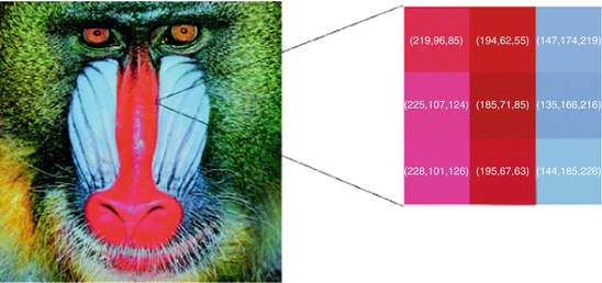
The nine pixels in the baboon image on the right have been enlarged. They present a high red-blue contrast. In the red pixels, the first (red) component is stronger. In the blue pixels, the third component, blue, dominates
The original sigma and neighborhood filter were proposed as an average of the spatially close pixels with a gray level difference lower than a certain threshold h. Thus, for a certain pixel x, the denoised value is the average of pixels in the spatial and intensity neighborhood:
 However, in order to make it coherent with further extensions and facilitate the mathematical development of this chapter, we will write the filter in a continuous framework under a weighted average form. We will denote the neighborhood or sigma filter by NF and define it for a pixel x as

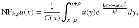
where B ρ (x) is a ball of center x and radius ρ > 0, h > 0 is the filtering parameter, and  is the normalization factor. The parameter h controls the degree of color similarity needed to be taken into account in the average. This value depends on the noise standard deviation σ, and it was set to 2. 5σ in [48] and [75].
(1)
is the normalization factor. The parameter h controls the degree of color similarity needed to be taken into account in the average. This value depends on the noise standard deviation σ, and it was set to 2. 5σ in [48] and [75].The Yaroslavsky and Lee’s filter (1) is less known than more recent versions, namely, the SUSAN filter [68] and the bilateral filter [70]. Both algorithms, instead of considering a fixed spatial neighborhood B ρ (x), weigh the distance to the reference pixel x:
where 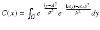 is the normalization factor and ρ > 0 is now a spatial filtering parameter. Even if the SUSAN algorithm was previously introduced, the whole literature refers to it as the bilateral filter. Therefore, we shall call this filter by the latter name in subsequent sections.
(2)
is the normalization factor and ρ > 0 is now a spatial filtering parameter. Even if the SUSAN algorithm was previously introduced, the whole literature refers to it as the bilateral filter. Therefore, we shall call this filter by the latter name in subsequent sections.The only difference between the neighborhood filter and the bilateral or SUSAN filter is the way the spatial component is treated. While for the neighborhood filter all pixels within a certain spatial distance are treated uniformly, for the bilateral or SUSAN filter, pixels closer to the reference one are considered more important. We display in Fig. 2 a denoising experience where a Gaussian white noise of standard deviation 10 has been added to a non-noisy image. We display the denoised image by both the neighborhood and bilateral filters. We observe that both filters avoid the excessive blurring caused by a Gaussian convolution and preserve all contrasted edges in the image.
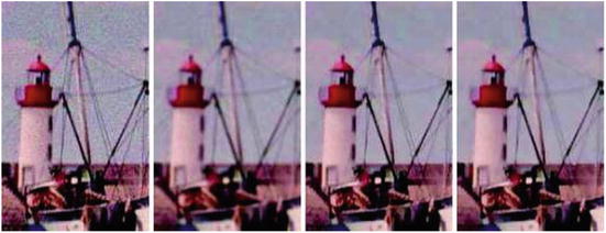
Fig. 2
From left to right: noise image, Gaussian convolution, neighborhood filter, and bilateral filter. The neighborhood and bilateral filters avoid the excessive blurring caused by a Gaussian convolution and preserve all contrasted edges in the image
The above denoising experience was applied to color images. In order to clarify how the neighborhood filters are implemented in this case, we remind that each pixel x is a triplet of values u(x) = (u 1(x), u 2(x), u 3(x)), denoting the red, green, and blue components. Then, the filter rewrites
 being the average of the distances of the three channels:
being the average of the distances of the three channels:The same definition applies for the SUSAN or bilateral filter by incorporating the spatial weighting term. The above definition naturally extends to multispectral images with an arbitrary number of channels. Bennett et al. [7] applied it to multispectral data with an infrared channel and Peng et al. [56] for general multispectral data.
The evaluation of the denoising performance of neighborhood filters and comparison with state-of-the-art algorithms are postponed to Sect. 2. In the same section, we present a natural extension of the neighborhood filter, the NL-means algorithm, proposed in [12]. This algorithm evaluates the similarity between two pixels x and y not only by the intensity or color difference of x and y but by the difference of intensities in a whole spatial neighborhood.
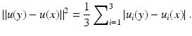
The bilateral filter was also proposed as a filtering algorithm with a filtering scale depending on both parameters h and ρ. Thus, taking several values for these parameters, we obtain different filtered images and corresponding residuals in a multi-scale framework. In Fig. 3, we display several applications of the bilateral filter for different values of the parameters h and ρ. We also display the differences between the original and filtered images in Fig. 4. For moderated values of h, this residual contains details and texture, but it does not contain contrasted edges. This contrasted information is removed by the bilateral filter only for large values of h. In that case, all pixels are judged as having a similar intensity level and the weight is set taking into account only the spatial component. It is well known that the residual by such an average is proportional to the Laplacian of the image. In Sect. 2, we will mathematically analyze the asymptotical expansion of the neighborhood residual image.
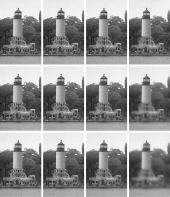
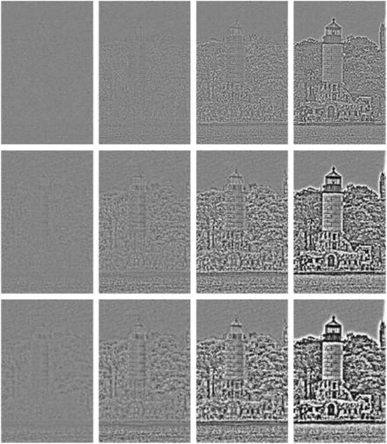
Fig. 3
Several applications of the bilateral filter for increasing values of parameters ρ and h. The parameter ρ increases from top to bottom taking values {2, 5, 10} and h increases from left to right taking values {5, 10, 25, 100}
Fig. 4
Residual differences between original and filtered images in Fig. 3. For moderated values of h this residual contains details and texture but it doesn’t contain contrasted edges. These contrasted information is removed by the bilateral filter only for large values of h
This detail removal of the bilateral while conserving very contrasted edges is the key in many image and video processing algorithms. Durand and Dorsey [28] use this property in the context of tone mapping whose goal is to compress the intensity values of a high-dynamic-range image. The authors isolate the details before compressing the range of the image. Filtered details and texture are added back at the final stage. Similar approaches for image editing are presented by Bae et al. [5], which transfer the visual look of an artist picture onto a casual photograph. Eisemann and Durand [32] and Petschnigg et al. [58] combine the filtered and residual image of a flash and non-flash image of the same scene. These two last algorithms, in addition, compute the weight configuration in one image of the pair and average the intensity values of the other image. As we will see, this is a common feature with iterative versions of neighborhood filters. However, for these applications, both images of the pair must be correctly and precisely registered.
The iteration of the neighborhood filter was not originally considered by the pioneering works of Lee and Yaroslavsky. However, recent applications have shown its interest. The iteration of the filter as a local smoothing operator tends to piecewise constant images by creating artificial discontinuities in regular zones. Barash et al. [6] showed that an iteration of the neighborhood filter was equivalent to a step of a certain numerical scheme of the classical Perona-Malik equation [57]. A complete proof of the equivalence between the neighborhood filter and the Perona-Malik equation was presented in [13] including a modification of the filter to avoid the creation of shocks inside regular parts of the image. Another theoretical explanation of the shock effect of the neighborhood filters can be found in Van de Weijer and van den Boomgaard [71] and Comaniciu [20]. Both papers show that the iteration of the neighborhood filter process makes points tend to the local modes of the histogram but in a different framework: the first for images and the second for any dimensional clouds of points. This discontinuity or shock creation in regular zones of the image is not desirable for filtering or denoising applications. However, it can be used for image or video editing as proposed by Winnemoller et al. [73] in order to simplify video content and achieve a cartoon look.
Even if it may seem paradoxical, linear schemes have showed to be more useful than nonlinear ones for iterating the neighborhood filter; that is, the weight distribution for each pixel is computed once and is maintained during the whole iteration process. We will show in Sect. 4 that by computing the weights on an image and keeping them constant during the iteration process, a histogram concentration phenomenon makes the filter a powerful segmentation algorithm. The same iteration is useful to linearly diffuse or filter any initial data or seeds as proposed by Grady et al. [38] for medical image segmentation or [11] for colorization (see Fig. 5 for an example). The main hypothesis for this seed diffusion algorithm is that pixels having a similar gray level value should be related and are likely to belong to the same object. Thus, pixels of different sites are related as in a graph with a weight depending on the gray level distance. The iteration of the neighborhood filter on the graph is equivalent to the solution of the heat equation on the graph by taking the graph Laplacian. Eigenvalues and eigenvectors of such a graph Laplacian can be computed allowing the design of Wiener and thresholding filters on the graph (see [69] and [59, 60] for more details).
Fig. 5
Colorization experiment using the linear iteration of the neighborhood filter. Top left: input image with original luminance and initial data on the chromatic components. Bottom right: result image by applying the linear neighborhood scheme to the chromatic components using the initial chromatic data as boundary conditions. Top middle and right: initial data on the two chromatic components. Bottom middle and bottom right: final interpolated chromatic components
Both the neighborhood filter and the NL-means have been adapted and extended for other types of data and other image-processing tasks: for 3D data set points [17, 26, 35, 43, 79], and [42]; demosaicking, the operation which transforms the “R or G or B” raw image in each camera into an “R and G and B” image [15, 51, 63]; movie colorization, [34] and [49]; image inpainting by proposing a nonlocal image inpainting variational framework with a unified treatment of geometry and texture [2] (see also [74]); zooming by a fractal-like technique where examples are taken from the image itself at different scales [29]; movie flicker stabilization [24], compensating spurious oscillations in the colors of successive frames; and super-resolution, an image zooming method by which several frames from a video, or several low-resolution photographs, can be fused into a larger image [62]. The main point of this super-resolution technique is that it gives up an explicit estimate of the motion, allowing actually for a multiple motion, since a block can look like several other blocks in the same frame. The very same observation is made in [30] for devising a super-resolution algorithm and in [22, 33].
2 Denoising
Analysis of Neighborhood Filter as a Denoising Algorithm
In this section, we will further investigate the neighborhood filter behavior as a denoising algorithm. We will consider the simplest neighborhood filter version which averages spatially close pixels with an intensity difference lower than a certain threshold h. By classical probability theory, the average of N random and i.i.d values has a variance N times smaller than the variance of the original values. However, this theoretical reduction is not observed when applying neighborhood filters.
In order to evaluate the noise reduction capability of the neighborhood filter, we apply it to a noise sample and evaluate the variance of the filtered sample. Let us suppose that we observe the realization of a white noise at a pixel x, n(x) = a. The nearby pixels with an intensity difference lower than h will be independent and identically distributed with the probability distribution function the restriction of the Gaussian to the interval  . If the research zone is large enough, then the average value will tend to the expectation of such a variable. Thus, the increase of the research zone and therefore of the number of pixels being averaged does not increase the noise reduction capability of the filter. Such a noise reduction factor is computed in the next result.
. If the research zone is large enough, then the average value will tend to the expectation of such a variable. Thus, the increase of the research zone and therefore of the number of pixels being averaged does not increase the noise reduction capability of the filter. Such a noise reduction factor is computed in the next result.Theorem 1.
Assume that the n(i) are i.i.d. with zero mean and variance σ 2. Then, the filtered noise by the neighborhood filter NFh satisfies the following:
The noise reduction depends only on the value of h,
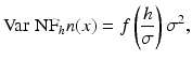
where
is a decreasing function with f(0) = 1 and limx→∞ f(x) = 0.
The values NFh n( x ) and NFh n( y ) are uncorrelated for x ≠ y .
The function f(x) is plotted in Fig. 6 . The noise reduction increases as the ratio h∕σ also does. We see that f(x) is near zero for values of x over 2.5 or 3, that is, values of h over 2.5σ or 3σ, which justifies the values proposed in the original papers by Lee and Yaroslavsky. However, for a Gaussian variable, the probability of observing values at a distance of the average larger than 2.5 or 3 times the standard deviation is very small. Thus, by taking these values, we excessively increase the probability of mismatching pixels of different objects. Thus, close objects with an intensity contrast lower than 3σ will not be correctly denoised. This explains the decreasing performance of the neighborhood filter as the noise standard deviation increases.
The previous theorem also tells us that the denoised noise values are still uncorrelated once the filter has been applied. This is easily justified since we showed that as the size ρ of the neighborhood increases, the filtered value tends to the expectation of the Gauss distribution restricted to the interval ( ). The filtered value is therefore a deterministic function of n(x) and h. Independent random variables are mapped by a deterministic function on independent variables.
). The filtered value is therefore a deterministic function of n(x) and h. Independent random variables are mapped by a deterministic function on independent variables.This property may seem anecdotic since noise is what we wish to get rid of. Now, it is impossible to totally remove noise. The question is how the remnants of noise look like. The transformation of a white noise into any correlated signal creates structure and artifacts. Only white noise is perceptually devoid of structure, as was pointed out by Attneave [3].
The only difference between the neighborhood filter and the bilateral or SUSAN filter is the way the spatial component is treated. While for the classical neighborhood all pixels within a certain distance are treated equally, for the bilateral filter, pixels closer to the reference pixel are more important. Even if this can seem a slight difference, this is crucial from a qualitative point of view, that is, the creation of artifacts.
It is easily shown that introducing the weighting function on the intensity difference instead of a non-weighted average does not modify the second property of Theorem 1, and the denoised noise values are still uncorrelated if ρ is large enough. However, the introduction of the spatial kernel by the bilateral or SUSAN filter affects this property. Indeed, the introduction of a spatial decay of the weights makes denoised values at close positions to be correlated.
There are two ways to show how denoising algorithms behave when they are applied to a noise sample. One of them is to find a mathematical proof that the pixels remain independent (or at least uncorrelated) and identically distributed random variables. The experimental device simply is to observe the effect of denoising on the simulated realization of a white noise. Figure 7 displays the filtered noises for the neighborhood filter, the bilateral filter, and other state-of-the-art denoising algorithms.
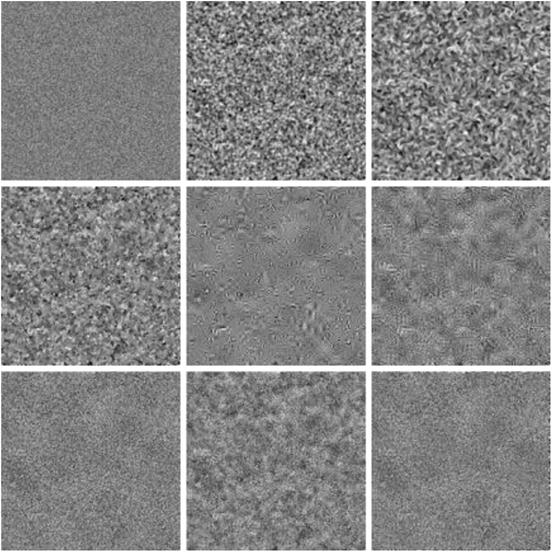
Fig. 7
The noise to noise criterion. From left to right and from top to bottom: original noise image of standard deviation 20, Gaussian convolution, anisotropic filtering, total variation, TIHWT, DCT empirical Wiener filter, neighborhood filter, bilateral filter, and the NL-means. Parameters have been fixed for each method so that the noise standard deviation is reduced by a factor 4. The filtered noise by the Gaussian filter and the total variation minimization are quite similar, even if the first one is totally blurred and the second one has created many high frequency details. The filtered noise by the hard wavelet thresholding looks like a constant image with superposed wavelets. The filtered noise by the neighborhood filter and the NL-means algorithm looks like a white noise. This is not the case for the bilateral filter, where low frequencies of noise are enhanced because of the spatial decay
Neighborhood Filter Extension: The NL-Means Algorithm
Now in a very general sense inspired by the neighborhood filter, one can define as “neighborhood of a pixel x” any set of pixels y in the image such that a window around y looks like a window around x. All pixels in that neighborhood can be used for predicting the value at x, as was shown in [23, 31] for texture synthesis and in [21, 80] for inpainting purposes. The fact that such a self-similarity exists is a regularity assumption, actually more general and more accurate than all regularity assumptions we consider when dealing with local smoothing filters, and it also generalizes a periodicity assumption of the image.
Let v be the noisy image observation defined on a bounded domain  , and let x ∈ Ω. The NL-means algorithm estimates the value of x as an average of the values of all the pixels whose Gaussian neighborhood looks like the neighborhood of x:
where G a is a Gaussian kernel with standard deviation a, h acts as a filtering parameter, and  is the normalizing factor. We recall that
 We will see that the use of an entire window around the compared points makes this comparison more robust to noise. For the moment, we will compare the weighting distributions of both filters. Figure 8 illustrates how the NL-means algorithm chooses in each case a weight configuration adapted to the local geometry of the image. Then, the NL-means algorithm seems to provide a feasible and rational method to automatically take the best of all classical denoising algorithms, reducing for every possible geometric configuration the mismatched averaged pixels. It preserves flat zones as the Gaussian convolution and straight edges as the anisotropic filtering while still restoring corners or curved edges and texture.
, and let x ∈ Ω. The NL-means algorithm estimates the value of x as an average of the values of all the pixels whose Gaussian neighborhood looks like the neighborhood of x:(3)
is the normalizing factor. We recall thatFig. 8
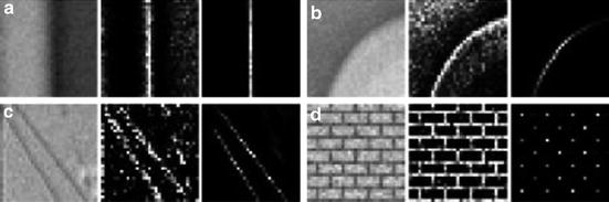
Weight distribution of NL-means, the bilateral filter, and the anisotropic filter used to estimate the central pixel in four detail images. On the two right-hand-side images of each triplet, we display the weight distribution used to estimate the central pixel of the left image by the neighborhood and the NL-means algorithm. (a) In straight edges, the weights are distributed in the direction of the level line (as the mean curvature motion). (b) On curved edges, the weights favor pixels belonging to the same contour or level line, which is a strong improvement with respect to the mean curvature motion. In the cases of (c) and (d), the weights are distributed across the more similar configurations, even though they are far away from the observed pixel. This shows a behavior similar to a nonlocal neighborhood filter or to an ideal Wiener filter
Due to the nature of the algorithm, one of the most favorable cases is the textural case. Texture images have a large redundancy. For each pixel, many similar samples can be found in the image with a very similar configuration, leading to a noise reduction and a preservation of the original image. In Fig. 9, one can see an example with a Brodatz texture. The Fourier transform of the noisy and restored images shows the ability of the algorithm to preserve the main features even in the case of high frequencies.
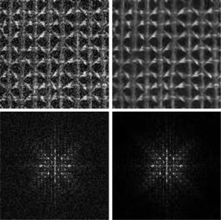
Fig. 9
NL-means denoising experiment with a Brodatz texture image. Left: noisy image with standard deviation 30. Right: NL-means restored image. The Fourier transforms of the noisy and restored images show how main features are preserved even at high frequencies
The NL-means seems to naturally extend the Gaussian, anisotropic, and neighborhood filtering. But it is not easily related to other state-of-the-art denoising methods as the total variation minimization [64], the wavelet thresholding [19, 27], or the local DCT empirical Wiener filters [76]. For this reason, we compare these methods visually in artificial denoising experiences (see [12] for a more comprehensive comparison).
Figure 10 illustrates the fact that a nonlocal algorithm is needed for the correct reconstruction of periodic images. Local smoothing filters and Wiener and thresholding methods are not able to reconstruct the wall pattern. Only NL-means and the global Fourier-Wiener filter reconstruct the original texture. The Fourier-Wiener filter is based on a global Fourier transform, which is able to capture the periodic structure of the image in a few coefficients. But this only is an ideal filter: the Fourier transform of the original image is being used. Figure 8d shows how NL-means chooses the correct weight configuration and explains the correct reconstruction of the wall pattern.
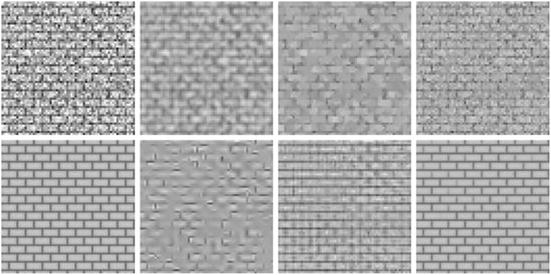
Fig. 10
Denoising experience on a periodic image. From left to right and from top to bottom: noisy image (standard deviation 35), Gauss filtering, total variation, neighborhood filter, Wiener filter (ideal filter), TIHWT (translation invariant hard thresholding), DCT empirical Wiener filtering, and NL-means
The NL-means algorithm is not only able to restore periodic or texture Images; natural images also have enough redundancy to be restored. For example, in a flat zone, one can find many pixels lying in the same region and with similar configurations. In a straight or curved edge, a complete line of pixels with a similar configuration is found. In addition, the redundancy of natural images allows us to find many similar configurations in faraway pixels.
Figure 11 shows that wavelet and DCT thresholding are well adapted to the recovery of oscillatory patterns. Although some artifacts are noticeable in both solutions, the stripes are well reconstructed. The DCT transform seems to be more adapted to this type of texture, and stripes are a little better reconstructed. For a much more detailed comparison between sliding window transform domain filtering methods and wavelet threshold methods, we refer the reader to [77]. NL-means also performs well on this type of texture, due to its high degree of redundancy.
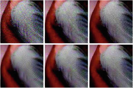
Fig. 11
Denoising experience on a natural image. From left to right and from top to bottom: noisy image (standard deviation 35), total variation, neighborhood filter, translation invariant hard thresholding (TIHWT), empirical Wiener, and NL-means
The above description of movie denoising algorithms and its juxtaposition to the NL-means principle shows how the main problem, motion estimation, can be circumvented. In denoising, the more samples we have the happier we are. The aperture problem is just a name for the fact that there are many blocks in the next frame similar to a given one in the current frame. Thus, singling out one of them in the next frame to perform the motion compensation is an unnecessary and probably harmful step. A much simpler strategy that takes advantage of the aperture problem is to denoise a movie pixel by involving indiscriminately spatial and temporal similarities (see [14] for more details on this discussion). The algorithm favors pixels with a similar local configuration, as the similar configurations move, so do the weights. Thus, the algorithm is able to follow the similar configurations when they move without any explicit motion computation (see Fig. 12).
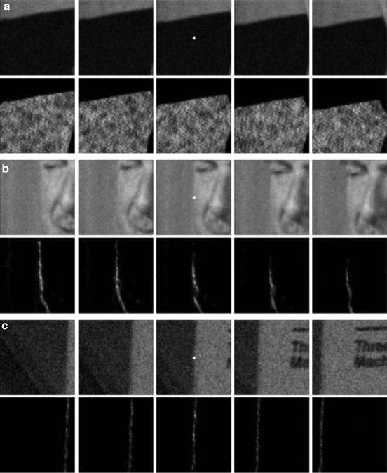
Fig. 12
Weight distribution of NL-means applied to a movie. In (a), (b), and (c), the first row shows a five frames image sequence. In the second row, the weight distribution used to estimate the central pixel (in white) of the middle frame is shown. The weights are equally distributed over the successive frames, including the current one. They actually involve all the candidates for the motion estimation instead of picking just one per frame. The aperture problem can be taken advantage of for a better denoising performance by involving more pixels in the average Fig. 7 displays the application of the denoising methods to a white noise. We display the filtered noise
Extension to Movies
Averaging filters are easily extended to the denoising of image sequences and video. The denoising algorithms involve indiscriminately pixels not belonging only to the same frame but also the previous and posterior ones.
In many cases, this straightforward extension cannot correctly deal with moving objects. For that reason, state-of-the-art movie filters are motion compensated (see [10] for a comprehensive review). The underlying idea is the existence of a “ground true” physical motion, which motion estimation algorithms should be able to estimate. Legitimate information should exist only along these physical trajectories. The motion compensated filters estimate explicitly the motion of the sequence by a motion estimation algorithm. The motion compensated movie yields a new stationary data on which an averaging filter can be applied. The motion compensation movie yields a new stationary data on which an averaging filter can be applied. The motion compensation neighborhood filter was proposed by Ozkan et al. [55]. We illustrate in Fig. 13 the improvement obtained with the proposed compensation.
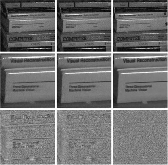
Fig. 13
Comparison of static filters, motion compensated filters, and NL-means applied to an image sequence. Top: three frames of the sequence are displayed. Middle and left to right: neighborhood filter, motion compensated neighborhood filter, and the NL-means. (AWA). Bottom: the noise removed by each method (difference between the noisy and filtered frame). Motion compensation improves the static algorithms by better preserving the details and creating less blur. We can read the titles of the books in the noise removed by AWA. Therefore, that much information has been removed from the original. Finally, the NL-means algorithm (bottom row) has almost no noticeable structure in its removed noise. As a consequence, the filtered sequence has kept more details and is less blurred
One of the major difficulties in motion estimation is the ambiguity of trajectories, the so-called aperture problem. This problem is illustrated in Fig. 14. At most pixels, there are several options for the displacement vector. All of these options have a similar gray level value and a similar block around them. Now, motion estimators have to select one by some additional criterion.
Fig. 14
Aperture problem and the ambiguity of trajectories are the most difficult problems in motion estimation: There can be many good matches. The motion estimation algorithms must pick one
3 Asymptotic
PDE Models and Local Smoothing Filters
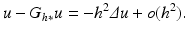
According to Shannon’s theory, a signal can be correctly represented by a discrete set of values, the “samples,” only if it has been previously smoothed. Let us start with u 0 the physical image, a real function defined on a bounded domain  . Then a blur optical kernel k is applied, i.e., u 0 is convolved with k to obtain an observable signal k ∗ u 0. Gabor remarked in 1960 that the difference between the original and the blurred images is roughly proportional to its Laplacian,
  . In order to formalize this remark, we have to notice that k is spatially concentrated and that we may introduce a scale parameter for k, namely,
 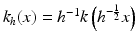 . If, for instance, u is C 2 and bounded and if k is a radial function in the Schwartz class, then
 Hence, when h gets smaller, the blur process looks more and more like the heat equation
 Thus, Gabor established a first relationship between local smoothing operators and PDEs. The classical choice for k is the Gaussian kernel.
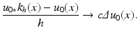
. Then a blur optical kernel k is applied, i.e., u 0 is convolved with k to obtain an observable signal k ∗ u 0. Gabor remarked in 1960 that the difference between the original and the blurred images is roughly proportional to its Laplacian, . In order to formalize this remark, we have to notice that k is spatially concentrated and that we may introduce a scale parameter for k, namely, . If, for instance, u is C 2 and bounded and if k is a radial function in the Schwartz class, thenRemarking that the optical blur is equivalent to one step of the heat equation, Gabor deduced that we can, to some extent, deblur an image by reversing the time in the heat equation,  . Numerically, this amounts to subtracting the filtered version from the original image:
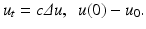
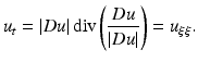
 This leads to considering the reverse heat equation as an image restoration, ill-posed though it is. The time-reversed heat equation was stabilized in the Osher-Rudin shock filter [54] who proposed
 where the propagation term
  is tuned by the sign of an edge detector Λ(u). The function Λ(u) changes sign across the edges where the sharpening effect therefore occurs. In practice, Λ(u) = Δ u and the equation is related to a reverse heat equation.
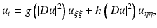
. Numerically, this amounts to subtracting the filtered version from the original image: is tuned by the sign of an edge detector Λ(u). The function Λ(u) changes sign across the edges where the sharpening effect therefore occurs. In practice, Λ(u) = Δ u and the equation is related to a reverse heat equation.The early Perona-Malik “anisotropic diffusion” [57] is directly inspired from the Gabor remark. It reads
 where
where  is a smooth decreasing function satisfying
  . This model is actually related to the preceding ones. Let us consider the second derivatives of u in the directions of Du and Du ⊥ :
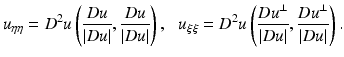 Then, Eq. (5) can be rewritten as
 where
where 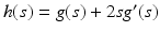 . Perona and Malik proposed the function
  . In this case, the coefficient of the first term is always positive and this term therefore appears as a one-dimensional diffusion term in the orthogonal direction to the gradient. The sign of the second coefficient, however, depends on the value of the gradient. When
  , this second term appears as a one-dimensional diffusion in the gradient direction. It leads to a reverse heat equation term when
 ![$$\vert \mathit{Du}\vert ^{2} > k$$” src=”/wp-content/uploads/2016/04/A183156_2_En_26_Chapter_IEq19.gif”></SPAN>.</DIV><br />
<DIV class=Para>The Perona-Malik model has got many variants and extensions. Tannenbaum and Zucker [<CITE><A href=]() 45] proposed, endowed in a more general shape analysis framework, the simplest equation of the list:
45] proposed, endowed in a more general shape analysis framework, the simplest equation of the list:
 This equation had been proposed some time before in another context by Sethian [66] as a tool for front propagation algorithms. This equation is a “pure” diffusion in the direction orthogonal to the gradient and is equivalent to the anisotropic filter AF [40]:
 where
where  and G h (t) denotes the one-dimensional Gauss function with variance h 2.
is a smooth decreasing function satisfying . This model is actually related to the preceding ones. Let us consider the second derivatives of u in the directions of Du and Du ⊥ :. Perona and Malik proposed the function . In this case, the coefficient of the first term is always positive and this term therefore appears as a one-dimensional diffusion term in the orthogonal direction to the gradient. The sign of the second coefficient, however, depends on the value of the gradient. When , this second term appears as a one-dimensional diffusion in the gradient direction. It leads to a reverse heat equation term when and G h (t) denotes the one-dimensional Gauss function with variance h 2.This diffusion is also related to two models proposed in image restoration. The Rudin-Osher-Fatemi [64] total variation model leads to the minimization of the total variation of the image  , subject to some constraints. The steepest descent of this energy reads, at least formally,
which is related to the mean curvature motion and to the Perona-Malik equation when 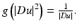 This particular case, which is not considered in [57], yields again (4). An existence and uniqueness theory is available for this equation [1].
, subject to some constraints. The steepest descent of this energy reads, at least formally,(4)
This particular case, which is not considered in [57], yields again (4). An existence and uniqueness theory is available for this equation [1].Asymptotic Behavior of Neighborhood Filters (Dimension 1)
Let u denote a one-dimensional signal defined on an interval  and consider the neighborhood filter
 where
where 
and consider the neighborhood filter The following theorem describes the asymptotical behavior of the neighborhood filter in 1D. The proof of this theorem and next ones in this section can be found in [13].
Theorem 2.
Suppose u ∈ C 2 (I), and let ρ,h,α > 0 such that ρ,h → 0 and h = 0(ρ α ). Consider the continuous function  , for
, for  , where
  . Let f be the continuous function
 Then, for


, for , where . Let f be the continuous function
Related posts:

Stay updated, free articles. Join our Telegram channel
Full access? Get Clinical Tree
