Spin Echo Imaging
Objectives
At the completion of this chapter, the student will be able to do the following:
Key Terms
Since the introduction in 1980 of clinically practical two-dimensional magnetic resonance imaging (MRI) followed shortly by multi-echo, multislice imaging, magnetic resonance (MR) image quality has continued to improve. In addition to better images, developments in MRI have been driven by the goal of reduced image acquisition time.
For instance, such reduced imaging time is required to image in the presence of normal tissue motion, including flowing blood (magnetic resonance angiography [MRA]). Figure 16-1 is a timeline representing the increase in temporal resolution of MRI since clinical introduction. Various tissue motion and MRI techniques are included on this timeline, along with the approximate dates of application of these techniques.
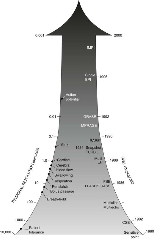
MRI development was predicted to follow a course similar to that of computed tomography (CT). An exponential introduction of new imaging techniques and clinical capabilities were expected up to a saturation point where the process would routinely remain clinical. Many predicted the death of CT because of the promise of MRI; however, MRI and CT are complementary in many respects. Advances in CT such as multislice spiral CT and computed tomography angiography (CTA) have extended the capabilities of CT.
MRI appears to be developing exponentially, not toward saturation but rather ever increasing. This chapter and the following five chapters describe the enormous advances in MRI temporal resolution. The term temporal resolution refers to resolution in time in the same way that spatial resolution refers to resolution in space and contrast resolution refers to resolution of one soft tissue from another.
 Improved temporal resolution requires faster imaging.
Although many of these MRI advances have resulted in faster imaging and increased patient throughput, they have also added new diagnostic capabilities. In addition to the imaging of cyclic motion such as respiration and heartbeat, noncyclic physiologic processes, such as peristalsis, saccadic eye motion, and joint movement, are being imaged with MRI. Furthermore, MR fluoroscopy (MRF) is now possible.
Even the first paper on nuclear magnetic resonance (NMR) by Felix Bloch in 1946 considered basic concepts leading to fast imaging techniques. The current development of fast and ultrafast imaging has been accompanied by an abundance of acronyms by vendors (Table 16-1). Each technique is a development of spin echo (SE) or gradient echo (GRE) imaging.
TABLE 16-1
Acronyms Used in Spin Echo and Gradient Echo Imaging
| Acronym | Explanation |
| BASG | Balanced SARGE |
| CE-FFE-T1 | Contrast-enhanced T1-weighted FFE |
| CE-FFE-T2 | Contrast-enhanced T2-weighted FFE |
| CISS | Constructive interference in the steady state |
| FAST | Fourier acquired steady state |
| FE | Field echo |
| bFFE | Balanced FFE |
| FFE | Fast field echo |
| FGR | Fast GRASS |
| FIESTA | Fast imaging employing steady state acquisition |
| FISP | Fast imaging with steady state precision |
| FLAIR | Fluid attenuated inversion recovery |
| FLASH | Fast low-angle shot |
| FSE | Fast spin echo |
| GFE | Gradient field echo |
| GRASS | Gradient recalled acquisition in the steady state |
| HASTE | Half Fourier acquired single shot turbo spin echo |
| HFI | Half Fourier imaging |
| IR | Inversion recovery |
| MPGR | Multiplanar GRASS |
| MPRAGE | Magnetization prepared rapid gradient echo |
| PFI | Partial flip angle |
| PSIF | Reversed FISP |
| RARE | Rapid acquisition by repeated echo |
| RASE | Rapid acquired spin echo |
| RF-FAST | RF-spoiled FAST |
| SARGE | Spoiled steady state acquisition rewinded gradient echo |
| SPGR | Spoiled GRASS |
| SSFP | Steady state free precession |
| STIR | Short time inversion recovery |
| TFE | Turbo field echo |
| True FISP | Balanced SSFP |
| True SSFP | Balanced SSFP |
| TSE | Turbo spin echo |
| TurboFLASH | Version of FLASH with IR spin preparation |
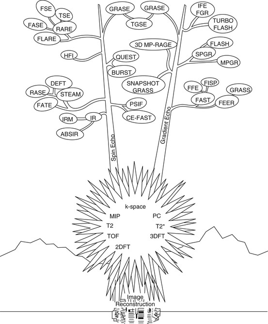
A rare, two-stalk century plant found in the Big Bend region of west Texas is shown in Figure 16-2. The root spines represent MR image reconstruction methods and the flowering pods represent imaging techniques.
Spin Echo Pulse Sequence
The most commonly used MRI technique is based on the SE pulse sequence that was introduced in 1950 by Hahn. This was first applied to imaging in 1980 and was quickly followed by additional modifications in the pulse sequence to allow multislice imaging. The Carr-Purcell-Meiboom-Gill (CPMG) pulse sequence is an improved SE pulse sequence for producing images from multiple echoes.
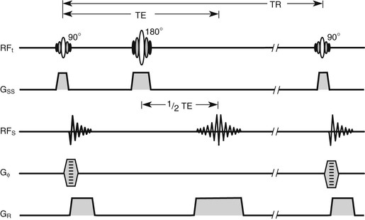
The terms radiofrequency (RF) pulse sequence and pulse sequence are often used interchangeably. However, RF pulse sequence correctly applies only to the first line of the musical score. Therefore the term pulse sequence is used here to represent not only the RF pulses but also the pulsed gradient magnetic fields and the received MR signals. The basic SE pulse sequence is shown in Figure 16-3.
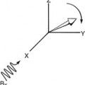
Often the lines of the musical score are identified as RFt, GZ, RFS, GY(Φ), and GX(ω) (Figure 16-4, A). These symbols identify images that are acquired in the transverse plane. Other orthogonal and oblique planes are now frequently obtained, so the symbols GZ, GY, and GX are less meaningful.
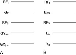
In this and successive chapters, the following symbols are used: RFt, GSS, RFs, Bф, and GR (Figure 16-4, B). In practice, any of the physical (x, y, or z) gradient coils can perform the functions of slice selection, phase encoding, or freqeuncy encoding. Thus, these symbols are more appropriate for indicating the functional utility of gradient magnetic fields.
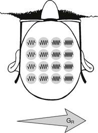
The slice selection gradient is represented by GSS, which can define any of the three orthogonal planes. Oblique images are obtained when GSS represents any combination of the three gradients energized simultaneously. The phase-encoding gradient magnetic field is Gф. The gradient magnetic field that is energized while a signal is acquired is GR, the read gradient. Sometimes GR is identified as the frequency-encoding gradient magnetic field.
The GSS is energized to establish a difference in resonance frequency along one axis. Usually, it is the long axis of the patient lying supine if transverse images are required. An RF pulse covering a specified frequency range excites proton spins in a slice of the patient.
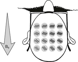
The transverse magnetization of the patient (MXY) is then phase encoded, using Gф, in a direction perpendicular to the long axis of the patient, along either the anterior-posterior axis (Y) or the lateral axis (X). This phase encoding is accomplished by briefly energizing either the X or Y gradient coils. When the phase-encoding gradient magnetic field is off, all spins precess with the same frequency but now have different phase shifts that depend on position along the phase-encoding gradient.
 Frequency encoding of the MRI signal helps locate that signal in the patient.
Next, the remaining gradient magnetic field, GR, is switched on for a well-defined interval, during which time the MR signal is received. During this time interval, a difference in resonance frequencies along the direction of frequency encoding occurs, causing the transverse magnetization to rotate with different frequency depending on location along that axis (Figure 16-5). This is often termed frequency encoding.
The commonly used reconstruction algorithms can distinguish between phase positions of opposite sign. The phase-encoding gradient has to be of a defined amplitude and time duration to distinguish between adjacent voxels (Figure 16-6).
Unfortunately, with just one phase gradient amplitude, an ambiguous signal is received. The solution, as discussed in Chapters 12 through 14, requires that this pulse sequence be repeated with a number of different phase-encoding amplitudes equal to the required matrix size.
During the time between the 90° and 180° RF pulses, the spin-spin or transverse relaxation causes a dephasing of the transverse magnetization. Other mechanisms, such as magnetic field inhomogeneities, varying magnetic susceptibility of different tissues, and chemical shift, also contribute to the dephasing of MXY during this time.
The 180° RF refocusing pulse inverts the phase of the spins by putting the faster component of the transverse magnetization behind the slower. This effect should persist over time, except the dephasing caused by nonrandom processes, such as static magnetic field, B0 inhomogeneity. Inhomogeneity is refocused after the 180° RF pulse to form the SE.
 When refocusing is provided by a 180° RF pulse, the pulse sequence is called a spin echo pulse sequence.
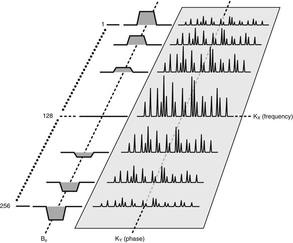
In SE imaging, the spatial frequency domain (k-space) is filled line by line in sequential order from bottom to top (Figure 16-7). This process normally starts with large, negative phase-encoding gradient amplitudes going through zero phase-encoding gradient amplitude and then to a large, positive phase-encoding gradient amplitude.
Related posts:


Stay updated, free articles. Join our Telegram channel

Full access? Get Clinical Tree


