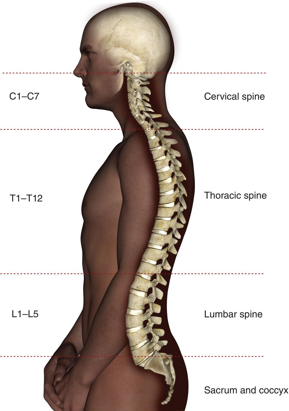
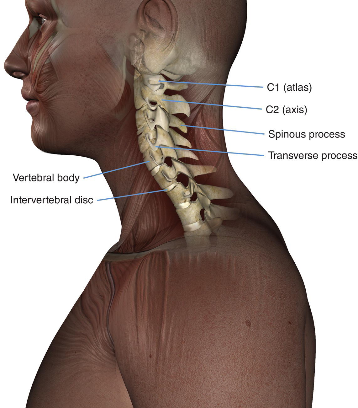
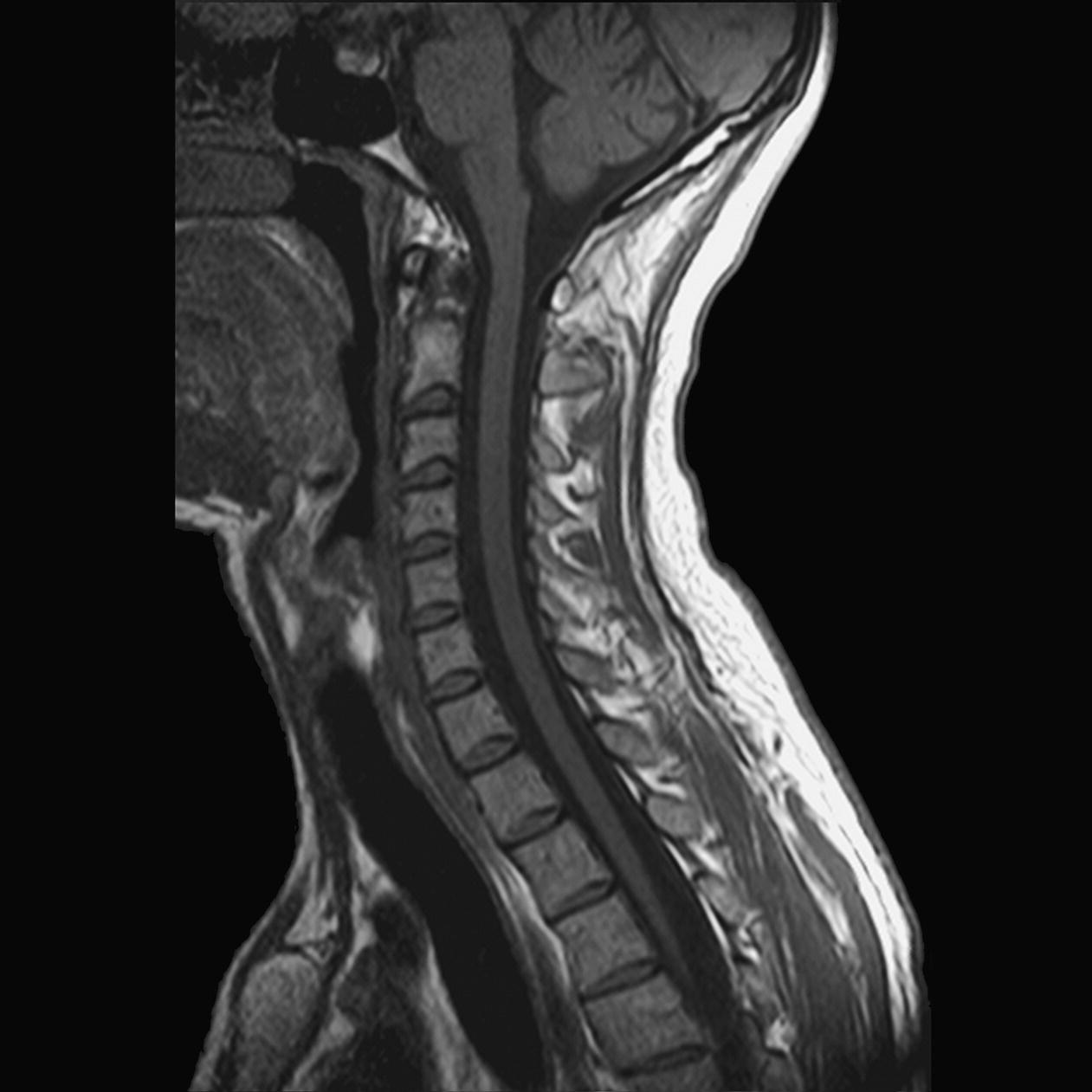
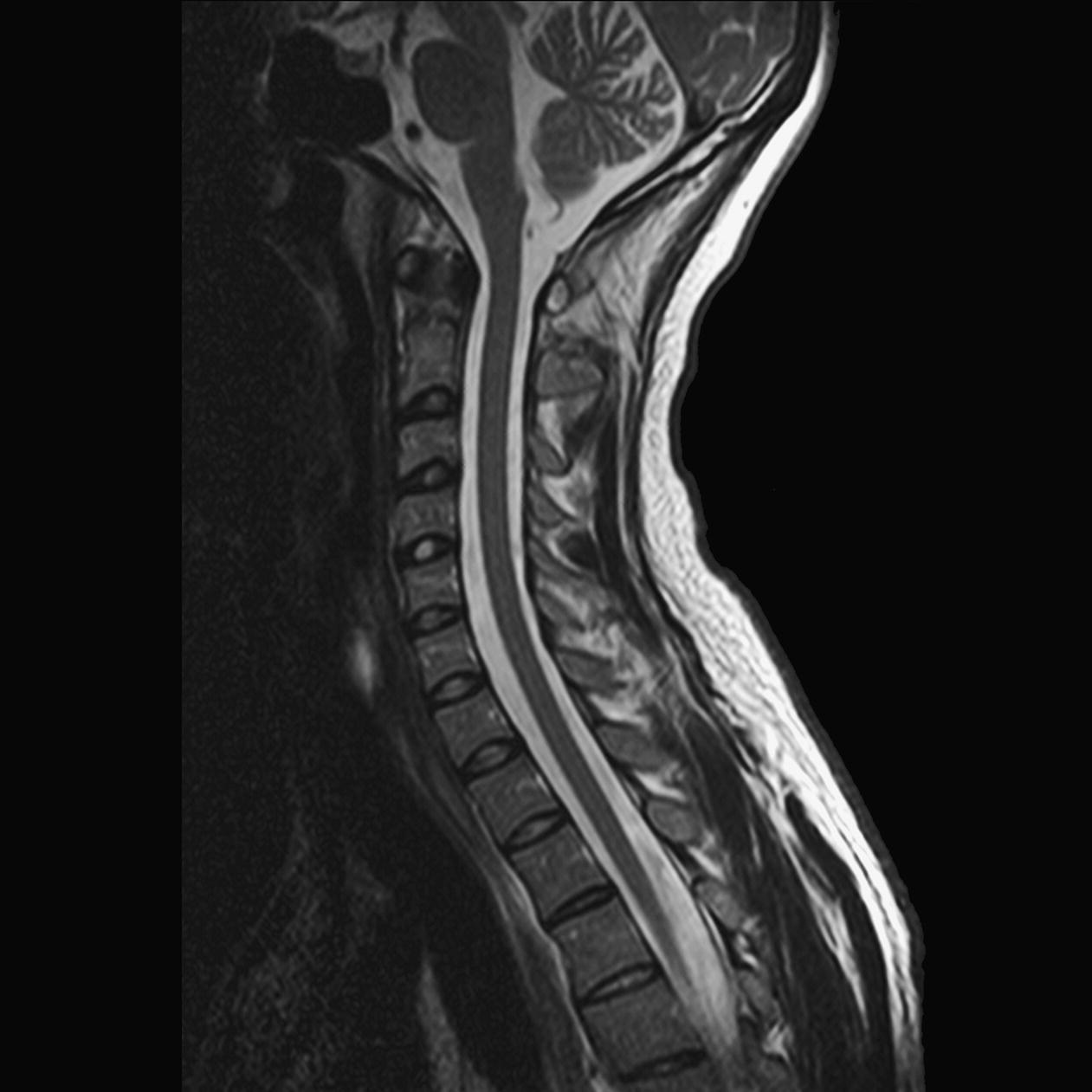
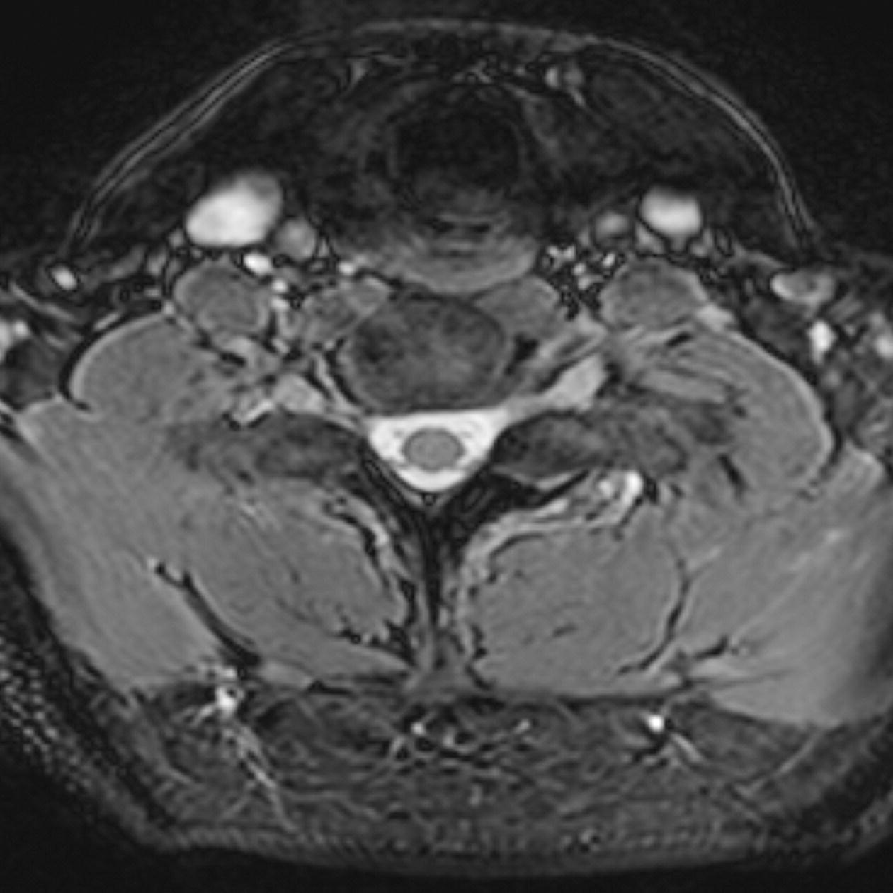
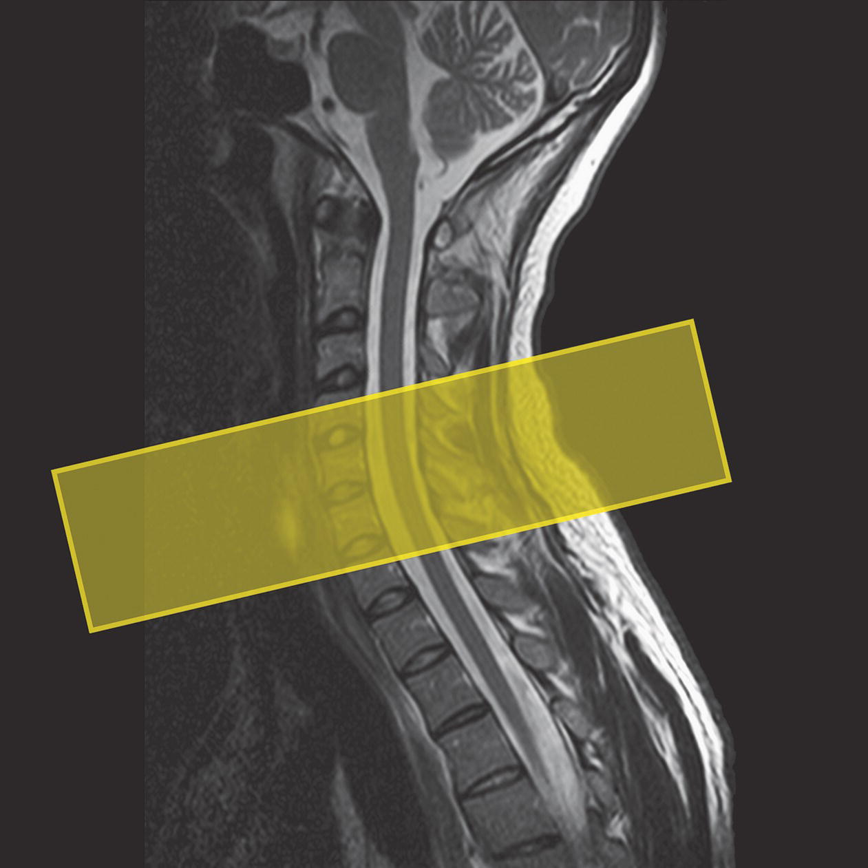
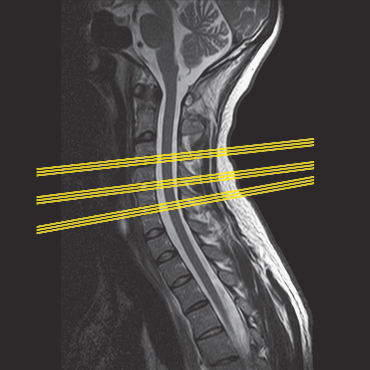
9 Table 9.1 Summary of parameters The figures given are for 1.5 T and 3 T systems. Parameters are dependent on field strength and may need adjustment for very low or very high field systems. Figure 9.1 Sagittal view of the spine showing vertebral levels. Figure 9.2 The components of the cervical spine and spinal cord. The patient lies supine on the examination couch with the neck coil placed under or around the cervical region. Coils are often moulded to fit the back of the head and neck so that the patient is automatically centred to the coil. If a flat coil is used, placing supporting pads under the shoulders flattens the curve of the cervical spine so that it is in closer proximity to the coil. The coil should extend from the base of the skull to the sterno-clavicular joints in order to include the whole of the cervical spine. The patient is positioned so that the longitudinal alignment light lies in the midline, and the horizontal alignment light passes through the level of the hyoid bone (this can usually be felt above the thyroid cartilage/Adam’s apple). The patient’s head is immobilized with foam pads and retention straps. Pe gating leads are attached if required. Acts as a localizer if three-plane localization is unavailable. The coronal or sagittal planes may be used. Coronal localizer: Medium slices/gaps are prescribed relative to the vertical alignment light, from the posterior aspect of the spinous processes to the anterior border of the vertebral bodies. The area from the base of the skull to the second thoracic vertebra is included in the image. P 20 mm to A 30 mm Sagittal localizer: Medium slice thickness/gaps are prescribed on either side of the longitudinal alignment light, from the left to the right lateral borders of the vertebral bodies. The area from the base of the skull to the second thoracic vertebra is included in the image. L 7 mm to R 7 mm Figure 9.3 Sagittal SE T1-weighted midline image through the cervical spine. Thin slices/gaps are prescribed on either side of the longitudinal alignment light, from the left to the right lateral borders of the vertebral bodies (unless the paravertebral areas are required). The area from the base of the skull to the second thoracic vertebra is included in the image. L 22 mm to R 22 mm Figure 9.4 Sagittal FSE T2-weighted midline image through the cervical cord. Slice prescription as for sagittal T1. Figure 9.5 Axial/oblique coherent GRE T2*-weighted image through the cervical cord. Thin slices/gaps are angled so that they are parallel to the disc space or perpendicular to the lesion under examination (Figures 9.6 and 9.7). For disc disease, three or four slices per level usually suffice. For larger lesions such as tumour or syrinx, thicker slices covering the lesion and a small area above and below may be necessary. Figure 9.6 Sagittal FSE T2-weighted image showing slice prescription boundaries and orientation for axial imaging of the cervical cord. Figure 9.7 Sagittal coherent GRE T2*-weighted image of the cervical spine showing axial/oblique slice positions parallel to each disc space. Slice prescription as for axial/oblique T2* with contrast enhancement for tumours. Slice prescription as for sagittal T2*. An alternative to coherent GRE T2*. A sagittal STIR may be useful for trauma to demonstrate muscular injuries. STIR sequences are typically much better than T2 FSE sequences for visualization of fractures and/or lesions in the vertebra. Additionally, MS plaques are almost always better visualized on a sagittal STIR sequence compared to an FSE T2-weighted sequence. Thin slices and a few or medium number of slice locations are prescribed through the ROI. If PD or T2* weighting is desired, then a coherent or steady-state sequence is utilized. If T1 weighting is required an incoherent or spoiled sequence is necessary. These sequences may be acquired in any plane but, if reformatting is required, isotropic data sets must be acquired. Slice prescription as for sagittal T1, T2 and T2*, except neck in flexion and extension to correlate the potential relevance of spondylotic changes to signs and symptoms. Figure 9.8 Axial balanced GRE through the cervical spine. The contrast characteristics of a BGRE sequence provide for high signal from CSF (high T2/T1 ratio) and thus produce images with high contrast between CSF and nerve roots. It is important to remember that because these images are not T2 weighted but rather weighted for the ratio of T1 to T2. Spins with a high T1 to T2 ratio appear bright (blood and CSF). Cord lesions such as MS plaques will not be seen. As such, they are typically utilized when imaging a patient for radiculopathy (disc disease) rather then myelopathy (cord lesions). The SNR in this region is mainly dependent on the quality of the coil. Posterior neck coils give adequate signal for the cervical spine and cord, but signal usually falls off at the anterior part of the neck, so they are not recommended for imaging structures such as the thyroid or larynx. In addition, flare from the posterior skin surface can be troublesome in sagittal T1 imaging, where the large fat pad situated at the back of the neck returns a high signal. Volume coils produce even distribution of signal, but the SNR in the cord is sometimes reduced compared with a posterior neck coil. Multi-coil array combinations commonly produce optimum SNR, and may be used with a large FOV to include the thoracic spine. This strategy is important when pathology extends from the cervical to the thoracic areas of the cord, for example, syrinx. Spatial resolution is also important, especially in axial/oblique imaging, as the nerve roots in the cervical region are notoriously difficult to visualize. Thin slices with a small gap and relatively fine matrices are employed to maintain spatial resolution. Ideally, 3D imaging is used as this allow very thin slices with no gap, and the volume may be viewed in any plane (see Volume imaging in Parameters and trade-offs in Part 1). Multiple NEX/NSA are also advisable if the inherent SNR is poor. Therefore, unless FSE is utilized, scan times are often of several minutes duration. Fortunately, a rectangular/asymmetric FOV is used very effectively in sagittal imaging as the cervical spine fits into a rectangle with its longitudinal axis running S to I. This facilitates the acquisition of fine matrices in short scan times. With a reduced FOV in the phase direction, aliasing may be a problem. In sagittal imaging, this artefact originates from the chin and the back of the head wrapping into the FOV. Increasing the size of the overall FOV or utilizing oversampling (if available) may eliminate or reduce this artefact. In addition, spatial pre-saturation pulses brought into the FOV to nullify signal coming from these structures are effective (see Flow phenomena and artefacts in Part 1). The multiple 180° RF pulses used in FSE sequences cause lengthening of the T2 decay time of fat so that the signal intensity of fat on T2-weighted FSE images is higher than in CSE. This sometimes makes the detection of marrow abnormalities difficult. Therefore, when imaging the vertebral bodies for metastatic disease, a STIR sequence should be utilized (see Pulse sequences in Part 1). The cervical area is often plagued with artefact. Not only does aliasing from structures outside the FOV obscure the image, but the periodic, pulsatile, motion of CSF within the spinal canal produces phase ghosting. The speed of flow is usually quite rapid in the cervical region, and therefore, conventional flow-reducing measures, such as spatial pre-saturation and GMN, are less effective than in the lumbar region where CSF flow is slower. On T1-weighted images, spatial pre-saturation pulses placed S and I to the FOV are usually sufficient. However, on T2-weighted sequences, flow artefact is commonly troublesome. In addition, selecting an S–I phase direction along with oversampling can also reduce CSF flow artefact in sagittal imaging and in that scenario, spatial pre-saturation pulses are not needed.
Spine
1.5 T
3 T
SE
SE
Short TE
Min–30 ms
Short TE
Min–15 ms
Long TE
70 ms+
Long TE
70 ms+
Short TR
600–800 ms
Short TR
600–900 ms
Long TR
2000 ms+
Long TR
2000 ms+
FSE
FSE
Short TE
Min–20 ms
Short TE
Min–15 ms
Long TE
90 +
Long TE
90 ms+
Short TR
400–600 ms
Short TR
600–900 ms
Long TR
4000 ms+
Long TR
4000 ms+
Short TEL
2–6
Short TEL
2–6
Long ETL
16+
Long ETL
16+
IR T1
IR T1
Short TE
Min–20 ms
Short TE
Min–20 ms
Long TR
3000 ms+
Long TR
300 ms+
TI
200–600 ms
TI
Short or null time of tissue
Short ETL
2–6
Short ETL
2–6
STIR
STIR
Long TE
60 ms+
Long TE
60 ms+
Long TR
3000 ms+
Long TR
3000 ms+
Short TI
100–175 ms
Short TI
210 ms
Long ETL
16+
Long ETL
16+
FLAIR
FLAIR
Long TE
80 ms+
Long TE
80 ms+
Long TR
9000 ms+
Long TR
9000 ms +(TR at least 4 × TI)
Long TI
1700–2500 ms (depending on TR)
Long TI
1700–2500 ms (depending on TR)
Long ETL
16+
Long ETL
16+
Coherent GRE
Coherent GRE
Long TE
15 ms+
Long TE
15 ms+
Short TR
<50 ms
Short TR
<50 ms
Flip angle
20–50°
Flip angle
20–50°
Incoherent GRE
Incoherent GRE
Short TE
Minimum
Short TE
Minimum
Short TR
<50 ms
Short TR
<50 ms
Flip angle
20–50°
Flip angle
20–50°
Balanced GRE
Balanced GRE
TE
Minimum
TE
Minimum
TR
Minimum
TR
Minimum
Flip angle
>40°
Flip angle
>40°
SSFP
SSFP
TE
10–15 ms
TE
10–15 ms
TR
<50 ms
TR
<50 ms
Flip angle
20–40°
Flip angle
20–40°
1.5 T and 3 T
Slice thickness 2D
Slice thickness 3D
Thin
2–4 mm
Thin
<1 mm
Medium
5–6 mm
Thick
>3 mm
Thick
8 mm
FOV
Matrix
Small
<18 cm
Coarse
256 × 128/256 × 192
Medium
18–30 cm
Medium
256 × 256/512 × 256
Large
>30 cm
Fine
512 × 512
Very fine
>1024 × 1024
NEX/NSA
Slice number 3D
Short
1
Small
<32
Medium
2–3
Medium
64
Multiple
>4
Large
>128
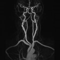
PC-MRA 2D and 3D
TOF-MRA 2D
TE
Minimum
TE
Minimum
TR
25–33 ms
TR
28–45 ms
Flip angle
30°
Flip angle
40–60°
VENC venous
20–40 cm/s
VENC arterial
60 cm/s
TOF-MRA 3D
TE
Minimum
TR
25–50 ms
Flip angle
20–30°
Cervical spine
Basic anatomy (Figures 9.1 and 9.2)
Common indications
Equipment
Patient positioning
Suggested protocol
Sagittal/coronal SE/FSE T1 or coherent GRE T2*
Sagittal SE/FSE T1 (Figure 9.3)
Sagittal SE/FSE T2 or coherent GRE T2* (Figure 9.4)
Axial/oblique SE/FSE T1/T2 or coherent GRE T2* (Figure 9.5)
Additional sequences
Sagittal/axial oblique SE/FSE T1
Sagittal SE/FSE T2 or STIR
3D coherent/incoherent (spoiled) GRE T2*/T1
Sagittal SE/FSE T1 or fast incoherent (spoiled) GRE T1/PD
3D balanced gradient echo (BGRE) (Figure 9.8)
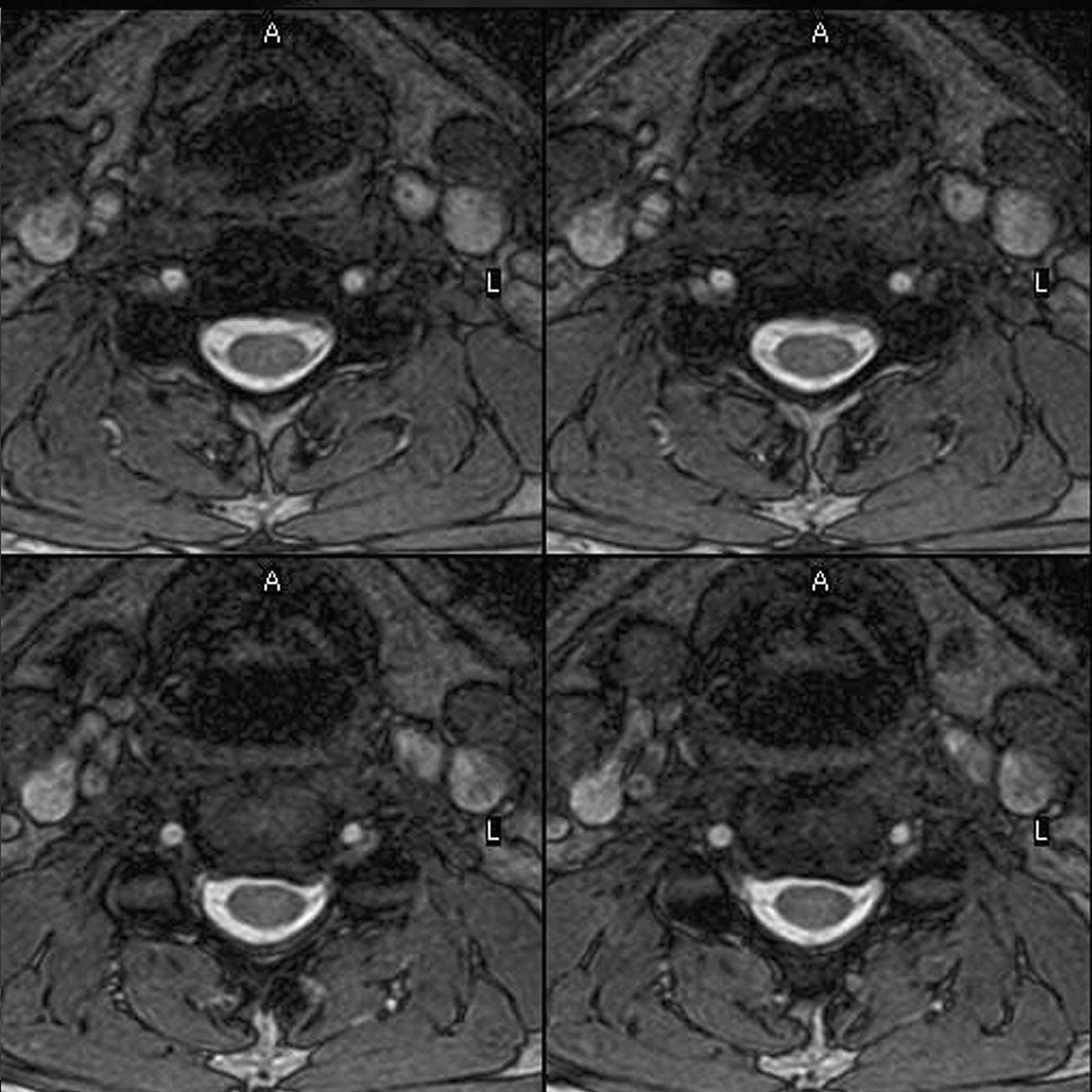
Image optimization
Technical issues
Artefact problems
Related posts:


Stay updated, free articles. Join our Telegram channel

Full access? Get Clinical Tree


