Sequence
TR (ms)
TE (ms)
Other parameters (TI, FA, ETL)
Slice thickness (mm)
No. of slices
FOV
Matrix
NEX
Examination time (min:s)

500
Min
–
6
16
24
256×192
1
1:23

500
Min
–
5
18
24
320×224
1
2:00

225
Min
FA 75
4
20
24
512×256
1
1:57

2075
24
TI auto
4
11×2
24
256×256
1
2:49

3000
88
ETL 12
6
21
24
256×224
2
2:24

4850
81
ETL 15
4
25
22
448×320
2
2:39

4975
85
ETL 15
3
25
20
512×320
4
7:20

8800
120
TI 2200
5
14×2
26
256×192
2
4:24

11,000
130
TI 2250
4
16×2
22
288×192
2
5:52
Lastly, two factors that depend on magnetic field strength need to be taken into consideration: the influence of the signal loss caused by the stronger susceptibility effects and the potentially diminished sensitivity of the radio-frequency coils at higher field intensity.
4.1.1 T1 Imaging
Since T1 relaxation times are longer at higher magnetic fields, entailing a reduction in the relative differences among different tissue types, it is generally difficult to obtain T1-weighted images with sufficient contrast when using a 3.0 T unit [2]. In fact, not only T1 increases, but the T1 values of different tissue types actually converge, giving rise to a narrower range of distribution. For this reason, optimization of the signal-to-noise ratio (SNR) in the same sample using a higher field unit requires longer TR (and a smaller flip angle), resulting in longer scanning times. Using longer TR, the gain in signal intensity in unit of time afforded by the higher magnetic field is therefore lost. T1 saturation for a given TR is greater at 3.0 T, resulting in reduced signal gain. In other words, the SNR per unit of time would be optimized with the shortest possible TR/T1. The possibility that the SNR gain connected with the high magnetic field may substantially be offset by a longer T1 highlights the importance of optimizing the imaging parameters [3].
The increased T1 is the main problem in 3.0 T brain imaging using SE T1-weighted sequences, which afford very unsatisfactory T1 contrast (Fig. 4.1) [7–10]. Indeed, the reduction in T1 differences among different types of tissues entails a loss of contrast between white and grey matter. For T1 contrast, this has led to the application of sequences other than SE which yield high T1 contrast irrespective of field strength, i.e. fast GE T1 (spoiled gradient echo, SPGR or MP-RAGE) and fast IR or fast FLAIR T1 weighted (Figs. 4.2, 4.3 and 4.4) [7–9].


Fig. 4.1
T1 imaging: comparison of the same SE T1 sequence (TR 500, 0.5 NEX, 1:00) acquired at 3.0 T (a) and 1.5 T (b). Note the less satisfactory white/grey matter contrast in (a)
Fig. 4.2
T1 imaging with SE T1 (a), FLAIR T1 (b) and FGRE T1 (c). The poor white/grey matter contrast of the SE T1 sequence (a) required performance of the other two high-contrast sequences. Note the typical high signal of the larger arterial vessels in (c) (arrow)
Fig. 4.3
(a–e) High-definition T1 images acquired with a 3D FSPGR IR-Prep sequence (750 ms, TR 8.4, TE 3.8, BW 50 kHz, FOV 160, matrix 416×320, slice thickness 2 mm). Coronal views (a–c, d, e) details
Fig. 4.4
High-definition images: comparison of a 3D FSPGR IR-Prep sequence (a, b) (TR 9.1, TE 4.0, FOV 170, slice thickness 2 mm, matrix 320×288) with an FSE-IR sequence (c, d) (TI 250 ms, FOV 160, slice thickness 3 mm, matrix 512×256). Note the optimum anatomical depiction of the cortico-subcortical junction on both sequences
Fast SPGR allows thinner slices to be obtained in a shorter time and provides images suitable for reformatting in all three planes using a single volumetric acquisition of the whole brain, thus disclosing a larger number of lesions than can be depicted using SE T1-weighted sequences acquired in a single plane. In addition, large arterial vessels appear hyperintense on fast SPGR sequences, although this does not impair image interpretation.
In contrast, fast IR entails longer scanning times because chained acquisitions are required to image the whole brain; this can be a problem when multiple unenhanced and contrast-enhanced studies, or different views, need to be performed.
Unlike IR T1-weighted sequences, which are less satisfactory and take longer to perform, a typical FLAIR T1-weighted study of the brain coupled with parallel imaging allows higher spatial resolution protocols to be applied in a shorter acquisition time.
Greater inflow contrast and enhanced background suppression make contrast-enhanced T1 imaging a definite advantage of 3.0 T systems. For instance, when studying primary and secondary brain tumours, the administration of a both single- and multiple-dose gadolinium yields greater contrast between tumour and normal brain tissue and allows the detection of more metastases and demonstrates different patterns of enhancement that may be useful to assess the degree of malignancy and to monitor response to therapy [11–13].
The greater sensitivity of 3.0 T contrast-enhanced investigations has also been demonstrated in multiple sclerosis, with a 21 %increase in the number of enhancing lesions detected, a 30 % increase in enhancing lesion volume and a 10 % increase in total lesion volume relative to scanning at 1.5 T [14].
Contrast-enhanced imaging also improves the evaluation of hypophyseal macro- and microadenomas (Figs. 4.5 and 4.6). 3.0 T MR venography is another valuable technique that provides increased spatial resolution, and thus more detailed information, in the same time of acquisition as a 1.5 T system [15].


Fig. 4.5
Unenhanced (a) and contrast-enhanced (b) hypophyseal microadenoma. PEI processing using Functool 2 (c)
Fig. 4.6
Hypophyseal macroadenoma: (a) unenhanced image (b) dynamic contrast-enhanced image
However, contrast-enhanced T1 semeiotics requires adjustments in TR and TE and a reduction in the dose of contrast agent [3]. The usual dosage of 0.1 mmol/kg can be halved without affecting image quality. Using a standard dose, the contrast/noise ratio (CNR) is two and a half times greater than with 1.5 T systems [15]. Double or triple doses can result in meningeal contrast uptake, a common non-pathological finding, at 3.0 T which at lower field strengths may, however, mimic carcinomatosis or meningitis and should thus be avoided.
To enhance sensitivity or highlight minimal changes in the blood-brain barrier, a double dose of contrast agent may be employed in selected investigations of brain metastases or inflammatory disease [16, 17]. In such cases, greater lesion enhancement with respect to normal brain parenchyma results in improved sensitivity and resolution.
Fast GE T1, rather than standard SE sequences, are preferred for contrast-enhanced T1 imaging, as they offer better contrast in the same acquisition time. SE T1 sequences are, however, consistently improved by contrast administration (Fig. 4.7).

Fig. 4.7
(a, b) Small left acoustic neurinoma: high-definition SE T1 sequence (matrix 512, thickness 1.5 mm). Unenhanced (a) and contrast-enhanced (b) images
4.1.2 T2 Imaging
In T2 contrast imaging, the advantages of high magnetic field strength are best exploited by performing fast SE sequences acquired using the same technique as with 1.5 T imagers but with shorter TR and TE due to the shorter T2 relaxation times (Fig. 4.8). High spatial resolution FSE-weighted images are especially effective at 3.0 T as they provide more anatomical detail and better contrast due to the greater SNR, which allows to employ thinner slices and broader matrices (Figs. 4.9, 4.10, 4.11, 4.12 and 4.13) [7–9, 18]. Even better images are obtained with inverted contrast FSE T2 sequences (Fig. 4.14).


Fig. 4.8
T2 imaging: comparison between the same FSE T2 sequence at 3.0 T (a, b zoom) and 1.5 T (c, d zoom). Anatomical detail and contrast resolution are greater in (a) and (b)
Fig. 4.9
High-definition FSE T2 image of the median sections of the brain
Fig. 4.10
High-definition FSE T2 image of the hippocampus
Fig. 4.11
High-definition FSE T2 image of the fifth cranial nerve in coronal (a), axial (b) and parasagittal (c) section
Fig. 4.12
(a, b) FSE T2 imaging. The excellent detail of this sequence allows visualization of the perivascular (Virchow-Robin) spaces at the level of the bi-hemispheric cortico-subcortical junction. Axial (a) and coronal (b) views
Fig. 4.13
Multiple sclerosis: (a–c) FSE T2 sequence
Fig. 4.14


High-definition FSE T2 sequence (matrix 512×320, thickness 3 mm, ZIP 1024) acquired with (a–c) and without (d–f) inverted contrast: coronal view. Note the excellent anatomical detail of both hippocampi
Related posts:

Stay updated, free articles. Join our Telegram channel
Full access? Get Clinical Tree
